The standard mass action kinetics model of gene expression arises from the differential equation \(df/dt = s - d f(t)\), with s being the constant synthesis rate, d the constant degradation rate and \(f0=f(0)\) (the abundance at time 0).
Arguments
- t
time in h
- s
synthesis date in U/h (arbitrary unit U)
- d
degradation rate in 1/h
- f0
the abundance at time t=0
Functions
f.old.equi(): abundance of old RNA assuming steady state (i.e. f0=s/d)f.old.nonequi(): abundance of old RNA without assuming steady statef.new(): abundance of new RNA (steady state does not matter)
Examples
d=log(2)/2
s=10
f.new(2,s,d) # Half-life 2, so after 2h the abundance should be half the steady state
#> [1] 14.42695
f.old.equi(2,s,d)
#> [1] 14.42695
s/d
#> [1] 28.8539
t<-seq(0,10,length.out=100)
plot(t,f.new(t,s,d),type='l',col='blue',ylim=c(0,s/d))
lines(t,f.old.equi(t,s,d),col='red')
abline(h=s/d,lty=2)
abline(v=2,lty=2)
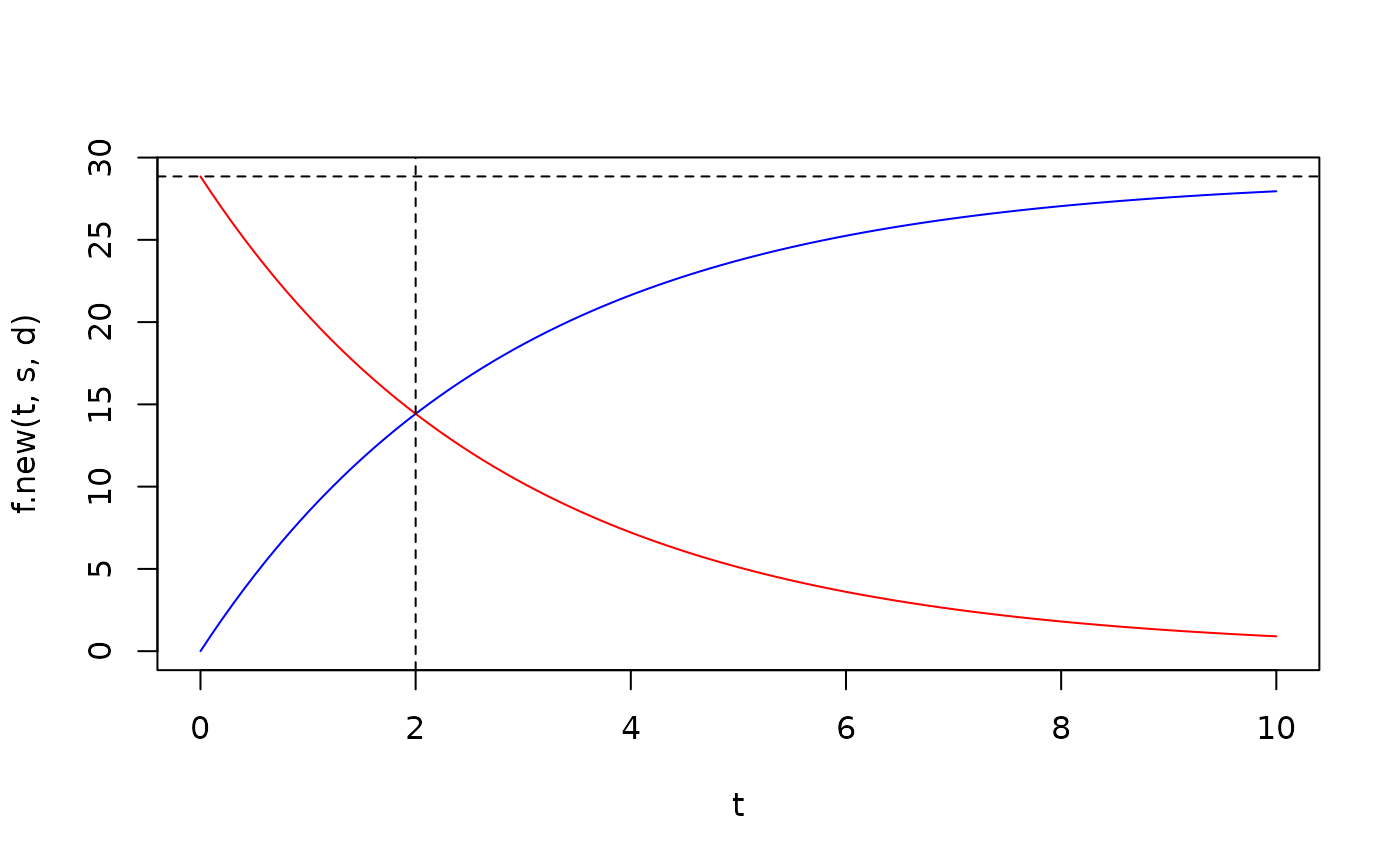 # so old and new RNA are equal at t=HL (if it is at steady state at t=0)
plot(t,f.new(t,s,d),type='l',col='blue')
lines(t,f.old.nonequi(t,f0=15,s,d),col='red')
abline(h=s/d,lty=2)
abline(v=2,lty=2)
# so old and new RNA are equal at t=HL (if it is at steady state at t=0)
plot(t,f.new(t,s,d),type='l',col='blue')
lines(t,f.old.nonequi(t,f0=15,s,d),col='red')
abline(h=s/d,lty=2)
abline(v=2,lty=2)
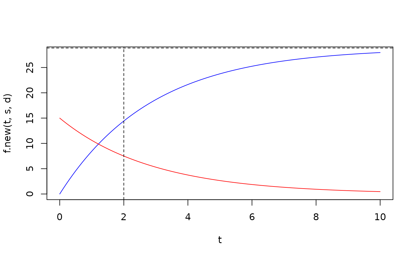 # so old and new RNA are not equal at t=HL (if it is not at steady state at t=0)