Analyzing Pulse-Chase Designs • grandR

This vignette will show the most suitable commands to work with pulse-chase data.

Throughout this vignette, we will be using the GRAND-SLAM processed SLAM-seq data set from Herzog et al. 2017 [1]. The data set includes SLAM-seq pulse-chase samples of mouse embryonic stem cells (mESCs) with pulse durations of 0, 0.5, 1, 3, 6, 12, and 24 hours.

suppressPackageStartupMessages({
  library(grandR)
  library(ggplot2)
  library(patchwork)
})

First we load the data and do the standard preprocessing steps. For more on these initial commands see the Loading data and working with grandR objects vignette.

In this step, we need to modify the sample names in the data, as the names were not processed using systematic naming conventions. If systematic sample names were used, the rename.sample parameter would not be necessary. This parameter allows us to specify a function for renaming the samples. The specified function removes all occurrences of “.chase” and replaces 0.5 with 0_5. For example, “mESC.0.5h.chase.B” becomes “mESC.0_5h.B” and “mESC.0h.chase.C” becomes “mESC.0h.C”. The output of the function is the modified vector after these replacements. This enables us to load the data using the design vector.

d=ReadGRAND("https://zenodo.org/record/7612564/files/chase_notrescued.tsv.gz?download=1",
            design=c(NA,"Time",Design$Replicate),
            rename.sample=function(v) 
              gsub(".chase","",gsub("0.5h","0_5h",v))
            )
d=FilterGenes(d)
d=Normalize(d)

The FitKinetics function can be utilized to analyze pulse-chase experiment data and estimate the synthesis and degradation rates of genes. To perform this analysis, the type parameter of the function should be set to “chase”. The function requires a grandR object as input, which holds the data from the pulse-chase experiment.

In addition to the required input, the FitKinetics function also has several optional parameters that allow for customization of the analysis. For further information on these parameters, please refer to the Kinetic modeling vignette.

The FitKinetics function uses the information in the grandR object and the specified parameters to fit a non-linear least squares model that describe the pulse-chase data. After fitting the models, the function returns a grandR object with an added analysis table that contains the inferred synthesis and degradation rates.

SetParallel()
d=FitKinetics(d,time="Time",type="chase")

The function GetAnalysisTable can be used to retrieve the results from this analysis.

head(GetAnalysisTable(d))

	Gene	Symbol	Length	Type	kinetics.Synthesis	kinetics.Half-life
Qsox1.155778412	Qsox1.155778412	Qsox1.155778412	258	Unknown	24.52101	3.450422
Ipo9.135384724	Ipo9.135384724	Ipo9.135384724	250	Unknown	42.98301	6.117657
Rpl37a.72713813	Rpl37a.72713813	Rpl37a.72713813	437	Unknown	180.89412	10.772538
Igfbp2.72852476	Igfbp2.72852476	Igfbp2.72852476	255	Unknown	215.53024	8.569694
Plekhb2.34879585	Plekhb2.34879585	Plekhb2.34879585	258	Unknown	35.69438	2.462591
Gmppa.75443176	Gmppa.75443176	Gmppa.75443176	252	Unknown	11.87146	6.073079

We can also visualize single genes graphically (this is the same gene as used in Fig 4a in Herzog et al. 2017 [1]):

PlotGeneProgressiveTimecourse(d,gene=Genes(d,"Dnmt3b",regex=TRUE),time="Time",type="chase")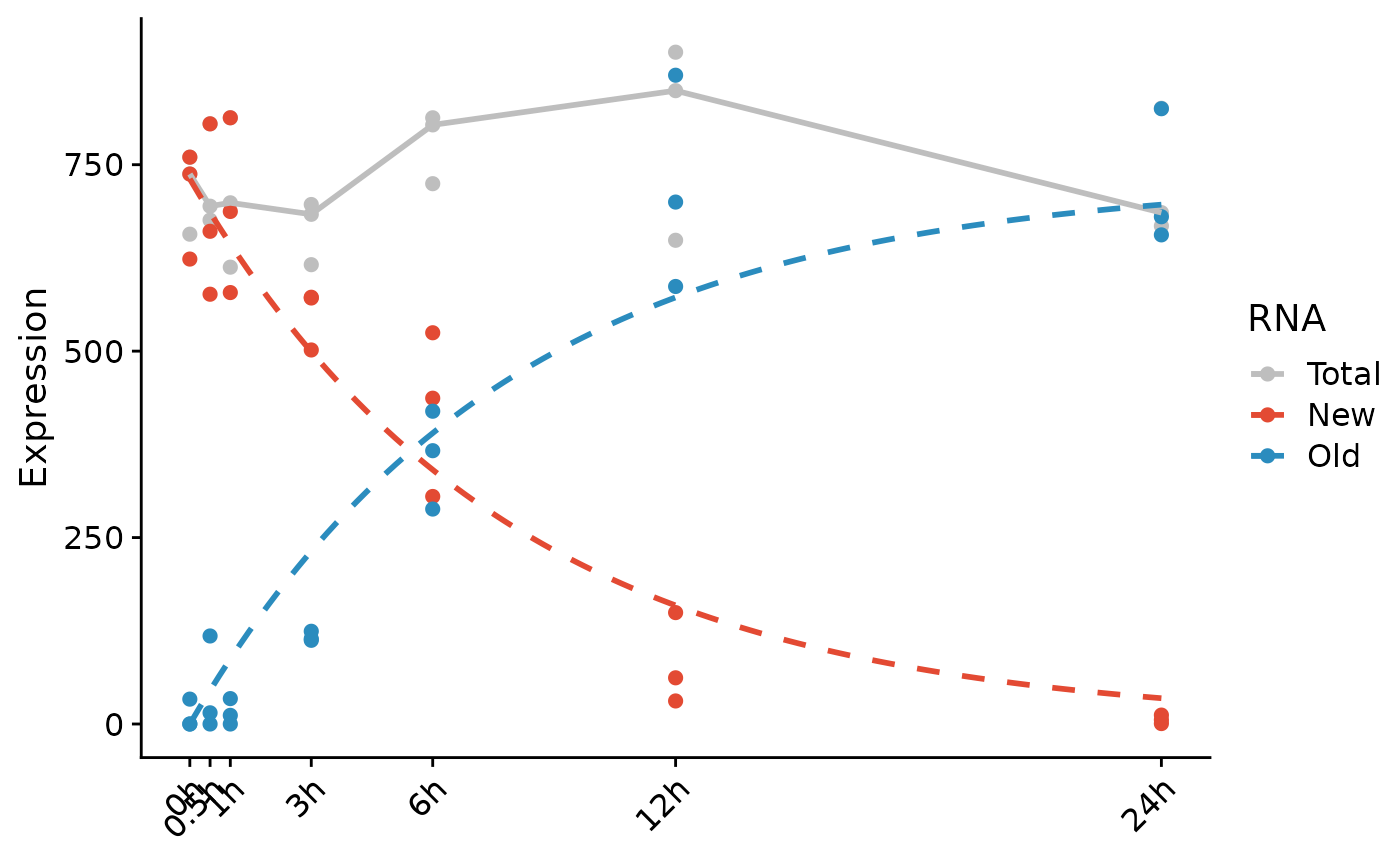

The curves represent the fitted model for this gene. Note that we do not specify the gene name directly, since here the gene names were labeled differently, and the Genes() function can be used to find the matching label:

Genes(d,"Dnmt3b",regex=TRUE)

[1] "Dnmt3b.153687730"

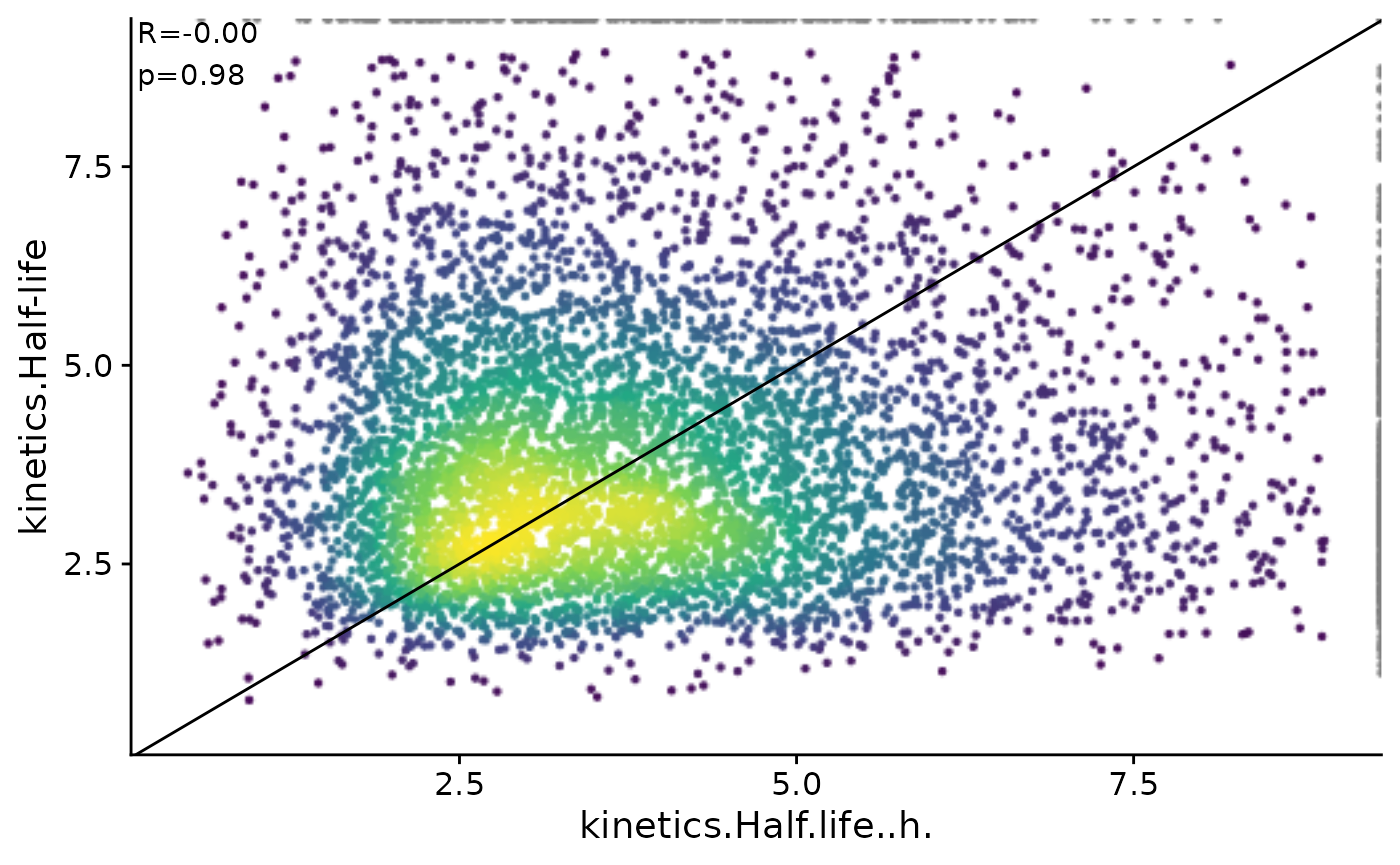
In this step, we compare the half-life values obtained from the FitKinetics function with those from Herzog et al. The latter was estimated by observing the decrease in mismatches during the chase period, while our method also considers the GRAND-SLAM-estimated NTR and posterior. To compare, we add Herzog et al’s half-life values to our analysis table and create a scatter plot with half-life values on both the x and y axes. The plot clearly shows a correlation between the two sets of results, indicating that the FitKinetics results are consistent with those from Herzog et al.

t=read.delim("https://zenodo.org/record/7612564/files/halflifes.tsv?download=1")
t$Gene=paste0(t$Name,".",t$End)
d = AddAnalysis(data = d,"kinetics",table = t,by="Gene")
PlotScatter(d,`kinetics.Half.life..h.`,`kinetics.Half-life`,
            correlation = FormatCorrelation())+geom_abline()