Loading single-cell data
Single-cell data in the form of feature-barcode matrices can be directly read into a grandR object. Two matrices must be prepared, one containing total counts, one containing new RNA counts. To demonstrate this, we will use publicly available data on cortisol response in single-cells of the A549 cell-line, including matrices of total and newly synthesized RNA (https://www.nature.com/articles/s41587-020-0480-9). The data is available on GEO under the accession ID GSM3770930.
First load the necessary packages.
suppressPackageStartupMessages({
    library(grandR)
    library(ggplot2)
    library(patchwork)
    library(Seurat)
})
Since we are downloading large files, the download may take some time. The default time limit in R is 60 seconds, which might be insufficient. We change increase the time limit as follows:
[1] 600Then we download the data and load them into grandR. The files
assigned to the genes,cells and
total.matrix is the normal matrix-market format that are
generated by most single cell processing pipelines (such as CellRanger
or STARsolo). Equivalently, genes,cells
andnew.matrix is a matrix-marked formatted matrix
containing counts of read with T-to-C mismatches.
Importantly, GRAND-SLAM output of single cell data can be read as
usual using the ReadGRAND function. The
detection.rate defines how many reads that truly originate
from labeled RNA have been recognized as such by having a T-to-C
mismatch. For details, see the sci-fate
paper. 82% is the value that has been estimated in this paper.
d <- ReadNewTotal(genes = "https://www.ncbi.nlm.nih.gov/geo/download/?acc=GSM3770930&format=file&file=GSM3770930%5FA549%5Fgene%5Fannotate%2Etxt%2Egz",
                  cells = "https://www.ncbi.nlm.nih.gov/geo/download/?acc=GSM3770930&format=file&file=GSM3770930%5FA549%5Fcell%5Fannotate%2Etxt%2Egz",
                  new.matrix = "https://www.ncbi.nlm.nih.gov/geo/download/?acc=GSM3770930&format=file&file=GSM3770930%5FA549%5Fgene%5Fcount%5Fnewly%5Fsynthesised%2Etxt%2Egz",
                  total.matrix = "https://www.ncbi.nlm.nih.gov/geo/download/?acc=GSM3770930&format=file&file=GSM3770930%5FA549%5Fgene%5Fcount%2Etxt%2Egz",
                  verbose=TRUE,
                  detection.rate = 0.82)
Downloading file (url: https://www.ncbi.nlm.nih.gov/geo/download/?acc=GSM3770930&format=file&file=GSM3770930%5FA549%5Fgene%5Fannotate%2Etxt%2Egz, destination: /tmp/RtmpWhRY7N/11721175982bf3) ...
Downloading file (url: https://www.ncbi.nlm.nih.gov/geo/download/?acc=GSM3770930&format=file&file=GSM3770930%5FA549%5Fcell%5Fannotate%2Etxt%2Egz, destination: /tmp/RtmpWhRY7N/1172115430f8ad) ...
Downloading file (url: https://www.ncbi.nlm.nih.gov/geo/download/?acc=GSM3770930&format=file&file=GSM3770930%5FA549%5Fgene%5Fcount%5Fnewly%5Fsynthesised%2Etxt%2Egz, destination: /tmp/RtmpWhRY7N/11721162a9857) ...
Downloading file (url: https://www.ncbi.nlm.nih.gov/geo/download/?acc=GSM3770930&format=file&file=GSM3770930%5FA549%5Fgene%5Fcount%2Etxt%2Egz, destination: /tmp/RtmpWhRY7N/1172119d8bf90) ...
Reading total count matrix...Warning: Duplicate gene symbols (n=141, e.g. SNORA18,SNORD67,snoU13,MIR3916,CRYBG3,PIK3R2)
present, making unique!Reading new count matrix...
Computing NTRs...
Deleting temporary file...
Deleting temporary file...
Deleting temporary file...
Deleting temporary file...Warning in grandR(prefix = genes$prefix, gene.info = gene.info, slots = re, : No no4sU entry
in coldata, assuming all samples/cells as 4sU treated!Now, d is a grandR object containing single cell
data:
dgrandR:
Read from https://www.ncbi.nlm.nih.gov/geo/download/
43167 genes, 7404 samples/cells
Available data slots: count,ntr
Available analyses:
Available plots:
Default data slot: countNote that also the cell meta-data has been loaded correctly, which is
the Coldata in grandR terms:
head(Coldata(d)) Name sample all_exon all_intron
sci-A549-001.ACTCTCTCAA sci-A549-001.ACTCTCTCAA sci-A549-001.ACTCTCTCAA 31785 6225
sci-A549-001.AAGAAGTTCA sci-A549-001.AAGAAGTTCA sci-A549-001.AAGAAGTTCA 31194 2514
sci-A549-001.ACGGAGAATA sci-A549-001.ACGGAGAATA sci-A549-001.ACGGAGAATA 17207 2270
sci-A549-001.CGATCCTGGA sci-A549-001.CGATCCTGGA sci-A549-001.CGATCCTGGA 14282 1932
sci-A549-001.ACTGAATTCC sci-A549-001.ACTGAATTCC sci-A549-001.ACTGAATTCC 32336 8779
sci-A549-001.GCCATCAACT sci-A549-001.GCCATCAACT sci-A549-001.GCCATCAACT 11058 4494
all_reads treatment_time doublet_score no4sU
sci-A549-001.ACTCTCTCAA 41737 4h 0.10704961 FALSE
sci-A549-001.AAGAAGTTCA 36264 6h 0.03695882 FALSE
sci-A549-001.ACGGAGAATA 21127 8h 0.04497354 FALSE
sci-A549-001.CGATCCTGGA 17723 4h 0.03797468 FALSE
sci-A549-001.ACTGAATTCC 44778 6h 0.07798960 FALSE
sci-A549-001.GCCATCAACT 17677 2h 0.03389831 FALSEPre-processing the data
We now could directly hand-over data to Seurat. However, pre-processing and analyses can also be performed in grandR. We filter genes such that only genes remain that have at least one UMI in at least 100 cells.
d <- FilterGenes(d, mode.slot = "count", minval = 1, mincol = 100)
d
grandR:
Read from https://www.ncbi.nlm.nih.gov/geo/download/
18276 genes, 7404 samples/cells
Available data slots: count,ntr
Available analyses:
Available plots:
Default data slot: countComputing new RNA percentage
We can also obtain some statistics, e.g. on the percentage of new RNA per cell, and the percentage of mitochondrial gene expression.
d <- ComputeExpressionPercentage(d,"percent.new",
                                 mode.slot="new.count",mode.slot.total="count")
d <- ComputeExpressionPercentage(d,"percent.mt",
                                 genes=Genes(d,"^MT-",regex=TRUE))
# results in 0 for all genes, have been filtered on GEO!
The computed percentages are now part of the coldata:
head(Coldata(d)) Name sample all_exon all_intron
sci-A549-001.ACTCTCTCAA sci-A549-001.ACTCTCTCAA sci-A549-001.ACTCTCTCAA 31785 6225
sci-A549-001.AAGAAGTTCA sci-A549-001.AAGAAGTTCA sci-A549-001.AAGAAGTTCA 31194 2514
sci-A549-001.ACGGAGAATA sci-A549-001.ACGGAGAATA sci-A549-001.ACGGAGAATA 17207 2270
sci-A549-001.CGATCCTGGA sci-A549-001.CGATCCTGGA sci-A549-001.CGATCCTGGA 14282 1932
sci-A549-001.ACTGAATTCC sci-A549-001.ACTGAATTCC sci-A549-001.ACTGAATTCC 32336 8779
sci-A549-001.GCCATCAACT sci-A549-001.GCCATCAACT sci-A549-001.GCCATCAACT 11058 4494
all_reads treatment_time doublet_score no4sU percent.new percent.mt
sci-A549-001.ACTCTCTCAA 41737 4h 0.10704961 FALSE 22.46687 0
sci-A549-001.AAGAAGTTCA 36264 6h 0.03695882 FALSE 16.48947 0
sci-A549-001.ACGGAGAATA 21127 8h 0.04497354 FALSE 19.02614 0
sci-A549-001.CGATCCTGGA 17723 4h 0.03797468 FALSE 18.97797 0
sci-A549-001.ACTGAATTCC 44778 6h 0.07798960 FALSE 30.89094 0
sci-A549-001.GCCATCAACT 17677 2h 0.03389831 FALSE 34.66831 0Here, the global percentage of new RNA correlates very well with the percentage of intronic reads in each cell (which is part of the table downloaded from GEO), i.e. there are two independent pieces of evidence that there are cells that are transcriptionally more active than others:
PlotScatter(Coldata(d),percent.new,all_intron/all_reads*100,
correlation = FormatCorrelation(),
remove.outlier = FALSE)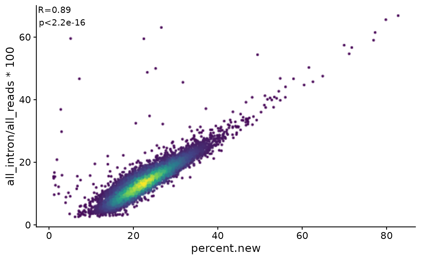 ``
``
Seurat
Data can be handed over to Seurat. For that, modalities and a mode must be defined. Allowed modalities are * total (total counts) * new (new counts) * old (old counts) * prev (estimated counts from the onset of labeling extrapolated using gene specific RNA half-lives)
The mode is one of four options (as outlined in this review): * assay: for each modality, the Seurat object will contain an assay * cells: cells are copied for each modality * genes: genes are copied for each modality * list: a list of Seurat objects is returned
Warning: Feature names cannot have underscores ('_'), replacing with dashes ('-')Warning: Data is of class dgTMatrix. Coercing to dgCMatrix.Warning: Feature names cannot have underscores ('_'), replacing with dashes ('-')
Warning: Feature names cannot have underscores ('_'), replacing with dashes ('-')
sAn object of class Seurat
36552 features across 7404 samples within 2 assays
Active assay: RNA (18276 features, 0 variable features)
1 layer present: counts
1 other assay present: newRNAThe percentage of new RNA could now be used as an additional QC filter:
VlnPlot(s,features = "percent.new",group.by = "treatment_time")Warning: Default search for "data" layer in "RNA" assay yielded no results; utilizing "counts"
layer instead.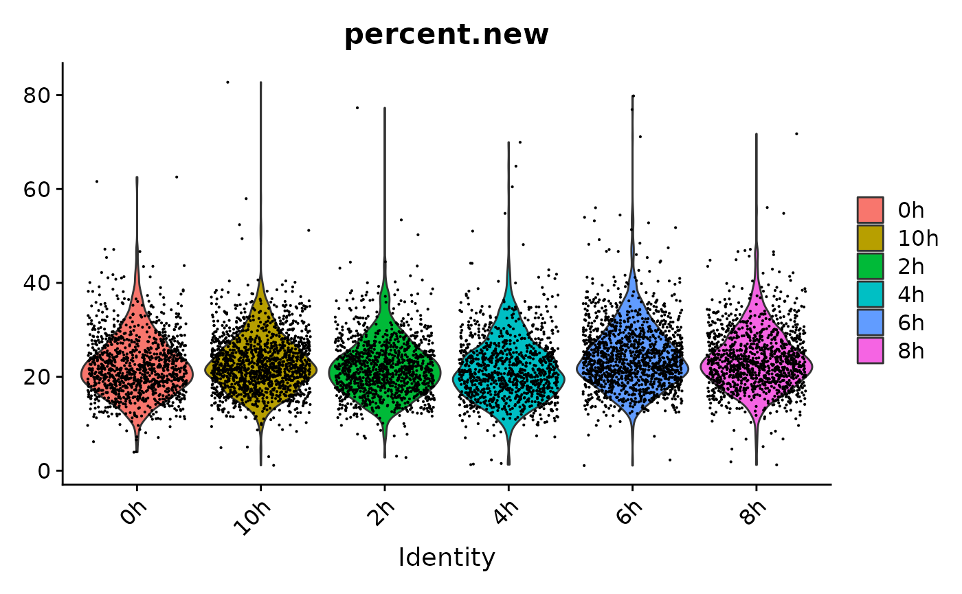
E.g. cells with extremely high amounts of new or old RNA could be filtered out. This step should only be done with care. Here we skip it, since the correlation with the percentage of intronic reads provides independent evidence that the high variance in new RNA content is biological.
Note that the new Seurat object has two assays, RNA and newRNA (which are the names we defined for the modalities). Let’s do the normal Seurat workflow for total RNA:
s <- NormalizeData(s)
s <- FindVariableFeatures(s)
s <- ScaleData(s)
s <- RunPCA(s,verbose = FALSE)
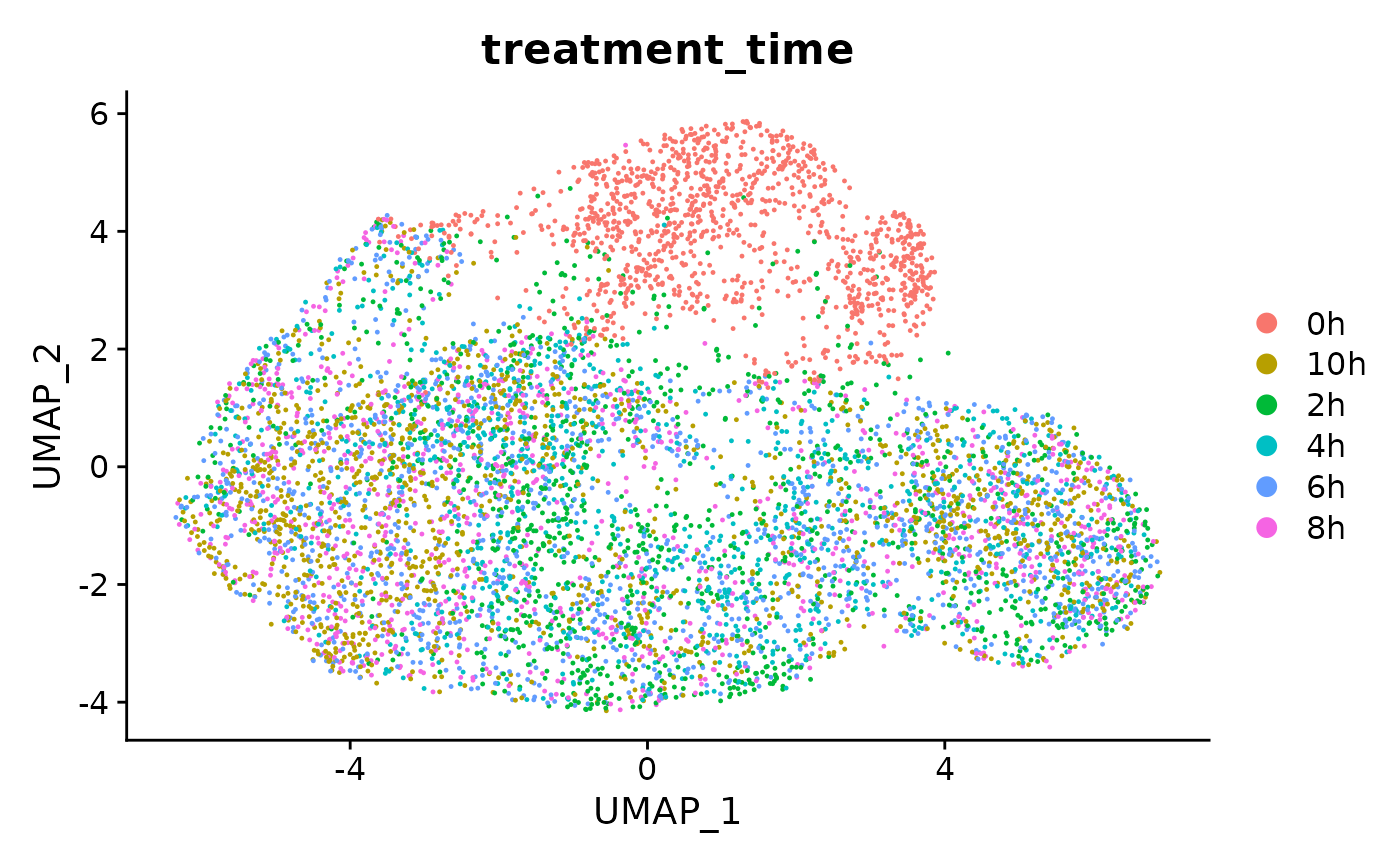
s <- RunUMAP(s,dims=1:10)
DimPlot(s,group.by = 'treatment_time') 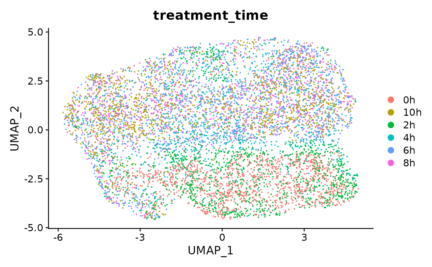
# treatment_time was transferred from the grandR Coldata table!And now repeat with new RNA:
DefaultAssay(s) <- 'newRNA'
s <- NormalizeData(s)
s <- FindVariableFeatures(s)
s <- ScaleData(s)
s <- RunPCA(s,verbose = FALSE)
s <- RunUMAP(s,dims=1:10)
DimPlot(s,group.by = 'treatment_time')