This vignette will show you the major steps and the workflow of Heterogeneity-seq. This will include trajectory generation and applying two Heterogeneity-seq methods.
The data we use here is originally from [Cao et al., 2020] and was reanalyzed in our [Heterogeneity-seq paper]. It is a scSLAM-seq time course data set of cells treated with the glucocorticoid Dexamethasone (DEX) for 10 hours with 2h labeling intervals.
First, we load in the HetSeq package alongside other useful packages as well as the preprocessed Seurat object:
suppressMessages({
library(HetSeq)
library(Seurat)
library(ggplot2)
library(ggrastr)
library(cowplot)
library(reshape2)
options(timeout = 600)
})

data <- readRDS(url("https://zenodo.org/records/14514453/files/dex_data.rds"))
Let’s have a look at the data:
DimPlot(data, group.by="treatmentTime")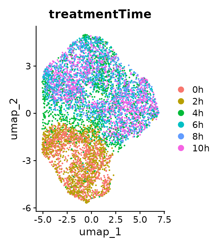
We can directly see that cells cluster differently according to the duration of DEX treatment. However, to investigate the expression strength of DEX response genes, we calculate a module score for each cell, using a list of DEX response genes used in the original study:
gc_genes <- readRDS(url("https://zenodo.org/records/14514453/files/gc_genes.rds"))
data$dex.percent <- AddModuleScore(data, list(dex.percent=intersect(rownames(data),gc_genes)), name = "DEX.modulescore", assay = "RNA")$DEX.modulescore1
data$dex.percent.new <- AddModuleScore(data, list(dex.percent=intersect(rownames(data),gc_genes)), name = "DEX.modulescore.new", assay = "newRNA")$DEX.modulescore.new1

df=as.data.frame(data@reductions$umap@cell.embeddings)
df$Condition=data$treatmentTime
df$dex.percent.new = data$dex.percent.new
ggplot(df, aes(x=umap_1,y=umap_2,color=dex.percent.new))+geom_point(size=0.2)+scale_color_viridis_c(option = "turbo", name="DEX score", limits=c(0,0.8), oob=scales::squish)+theme_cowplot()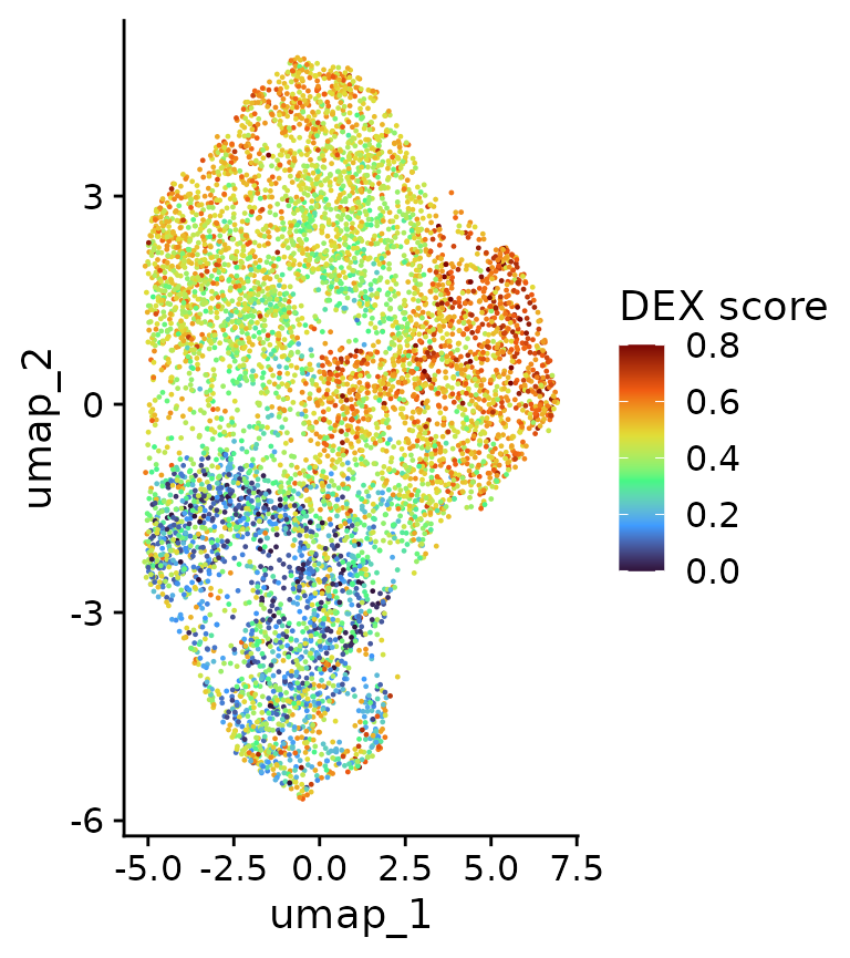
tab <- FetchData(data, c("treatmentTime", "dex.percent", "dex.percent.new"))
tab_melt <- melt(tab)
ggplot(tab_melt, aes(x=treatmentTime, y=value,color=variable))+geom_boxplot()+theme_cowplot()+theme(axis.title.x = element_blank())+
  scale_color_manual(values = c("#298c8c", "#800074"),labels = c("total RNA", "new RNA"))+ylab("DEX score")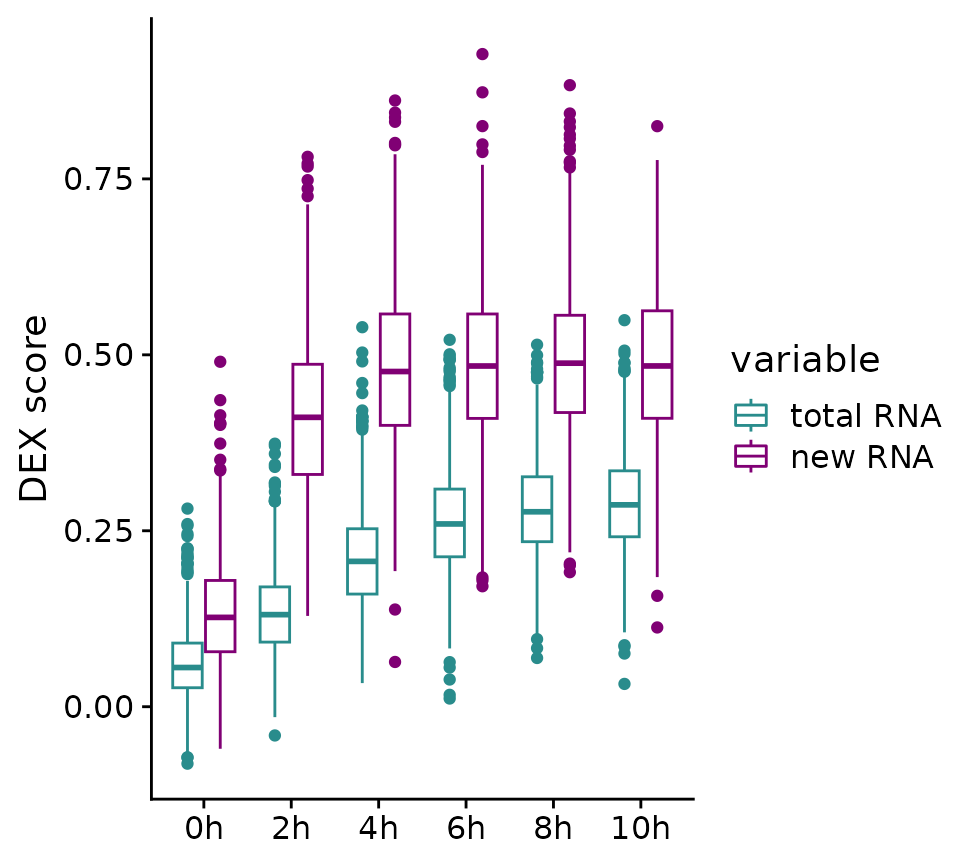
We can now see a strongly heterogeneous DEX response in cells from the same sample, both in total and in new RNA levels. These differences are likely based on intercellular heterogeneity at the start of DEX treatment and Heterogeneity-seq can leverage this information to identify the factors in old (or previous) RNA, which drive these outcomes. But first, we need to connect cells from an end point with distinguishable weak and strong responder cells back to control cells (0h). Theoretically, we could just use the last time point (10h) as the end point and the specific choice depends on the underlying biological pathway and the question asked. Here are two examples:
- Which factors drive a strong/quick initial response to DEX?
- Which factors determine a strong response in late time points?
If we look at the box plots of the DEX score in both new and total RNA, we see a continuously increasing score up to 6 or 8h in total RNA. Therefore, we could argue that these samples would be a suitable end point. However, looking at new RNA, we see a strong and heterogeneous initial response to DEX already after 2h and only minor to no increases afterwards. This makes the 2h sample a perfect end point to answer question 1. Choosing later time points is not necessary for this question and would lead to longer trajectories and could potentially add more noise. To answer question 2, the later time points would be suitable.
Let’s stick with the first question. To answer it, we need to first create trajectories from cells in the 2h time point back to their most likely predecessor in the control (0h) sample:
# Splitting the Seurat object into a list for convenience
treatment.list <- SplitObject(subset(data, subset = treatmentTime %in% c("0h", "2h")), split.by = "treatmentTime")

# distmat creates a distance matrix between cells from the 0h and the 2h sample. Distances are calculated between the total RNA (= "RNA") assay of the previous time point (0h) and the previous RNA (= "prevRNA") assay of the following time point.
D.list=list(
    distmat(treatment.list[["0h"]],treatment.list[["2h"]], "RNA", "prevRNA")
)
# Pruning the distance matrix to reduce the runtime of mincostflow. top.n parameter can be used to set a cutoff (10 by default)
D.list = prune(D.list, top.n = 10)

# Apply the min-cost-max-flow approach to generate optimal trajectories
trajectories = mincostflow(D.list)
Computing max flow...
max flow=1049, bottleneck=1049
Allocate 4208x17620 matrix...
Constructing capacity constraints for 2103 cells...
Constructing flow constraints and costs for 15517 edges...
Optimizing 17620 variables with 4208 constraints...
Constructing 1049 trajectories...
colnames(trajectories) <- c("0h", "2h")

# # Creating a full length trajectory would look like this:
# treatment.list <- SplitObject(data, split.by = "treatmentTime")
# D.list=list(
#     distmat(treatment.list[["0h"]],treatment.list[["2h"]], "RNA", "prevRNA"),
#     distmat(treatment.list[["2h"]],treatment.list[["4h"]], "RNA", "prevRNA"),
#     distmat(treatment.list[["4h"]],treatment.list[["6h"]], "RNA", "prevRNA"),
#     distmat(treatment.list[["6h"]],treatment.list[["8h"]], "RNA", "prevRNA"),
#     distmat(treatment.list[["8h"]],treatment.list[["10h"]], "RNA", "prevRNA")
# )
# D.list = prune(D.list)
# trajectories_10h = mincostflow(D.list)
# colnames(trajectories_10h) <- c("0h", "2h", "4h", "6h", "8h","10h")
With the trajectories generated, we can now call one of the Heterogeneity-seq approaches. Both HetseqClassify and HetseqDoubleML can either use the score.name or the score.group parameter to define groups in the end time point (here: 2h). score.name takes the name of a numeric metadata column in the Seurat object and automatically defines the response groups “Low”, “Middle” and “High”. These are by default based on the 0-25%, 25-75% and 75-100% quantiles but the cutoffs can be manually defined with the quantiles parameter. In contrast, score.group takes a named vector of response groups. With this, you can manually define response groups instead of relying on the quantile definition.
The classifier approach tries to predict either “Low” or “High” outcomes based on the expression of single genes at a time. Most genes will not be informative enough to result in high AUC values, but those that have high AUCs are likely candidate genes.
res_classify <- HetseqClassify(data, trajectories, score.name = "dex.percent.new", num_cores = 16)
 Low High
 263  262
PlotClassify(res_classify)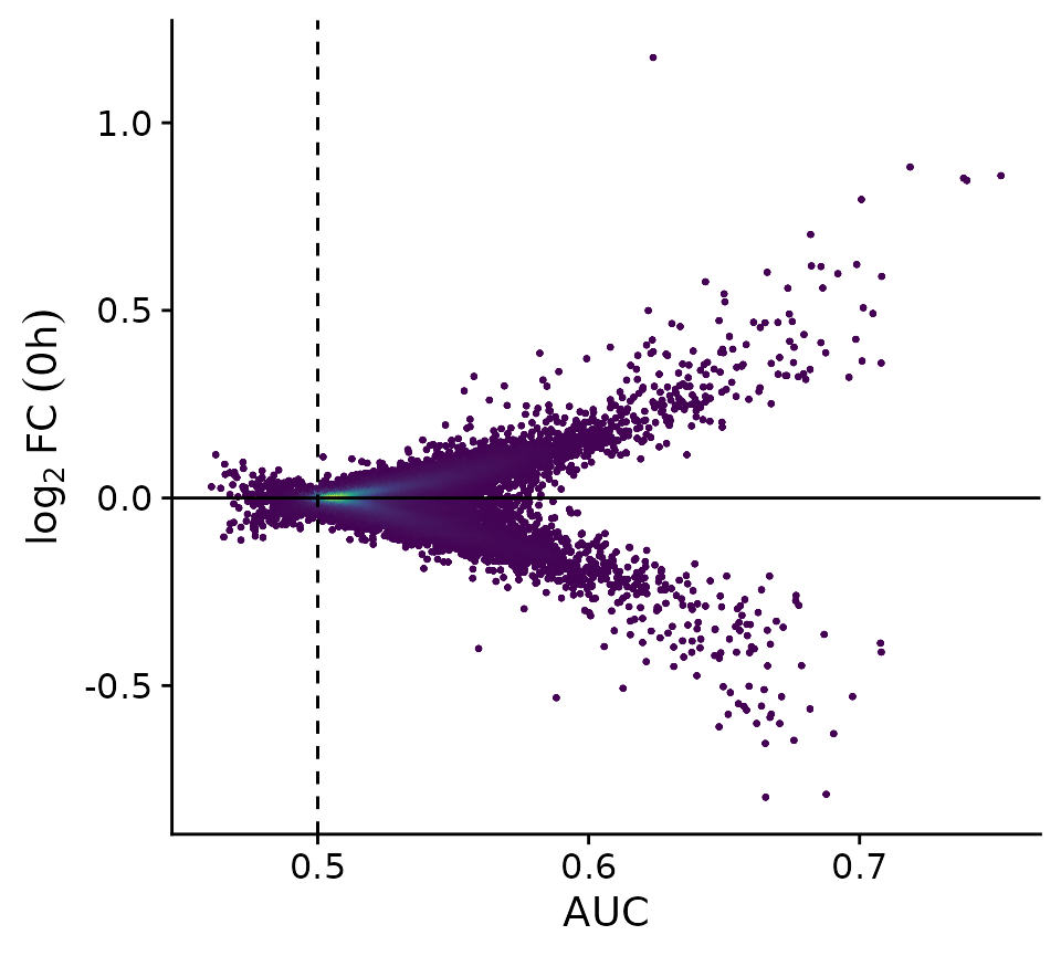
# Using score.group to achieve the same results
br1=quantile(data$dex.percent.new[trajectories$`2h`], probs = c(0.25))
br2=quantile(data$dex.percent.new[trajectories$`2h`], probs = c(0.75))
score.group = cut(data$dex.percent.new[trajectories$`2h`],breaks=c(-10,br1,br2,10),labels=c("Weak","Average","Strong"))


# When using a score.group with different levels than the default (Low, Middle, High), compareGroups has to be adapted to which levels should be compared.
# posClass can be set manually but will by default always be the second value in compareGroups.
res_classify_grp <- HetseqClassify(data, trajectories, score.group = score.group, compareGroups = c("Weak", "Strong"), posClass = "Strong", num_cores = 16)
Strong   Weak
   262    263
all.equal(res_classify$AUC, res_classify_grp$AUC)[1] TRUEThe results of the classifier gives us an extensive list of genes and how well their expression can be used to predict the cell fate of control cells. Genes with high AUC values have strong predictive power and are therefore likely candidates for modulating the DEX pathway. Gene Ontology Analysis can give us a closer look at these genes and if there are any coherent functional relationships.
suppressMessages({
  library(clusterProfiler)
  library(org.Hs.eg.db)
})

ego_down <- enrichGO(gene         = res_classify[res_classify$AUC>0.65 & res_classify$LFC<0,]$Gene,
                  OrgDb         = org.Hs.eg.db,
                  universe = res_classify$Gene,
                  keyType       = 'SYMBOL',
                  ont           = "BP",
                  pAdjustMethod = "BH",
                  pvalueCutoff  = 0.01,
                  qvalueCutoff  = 0.05)
barplot(ego_down)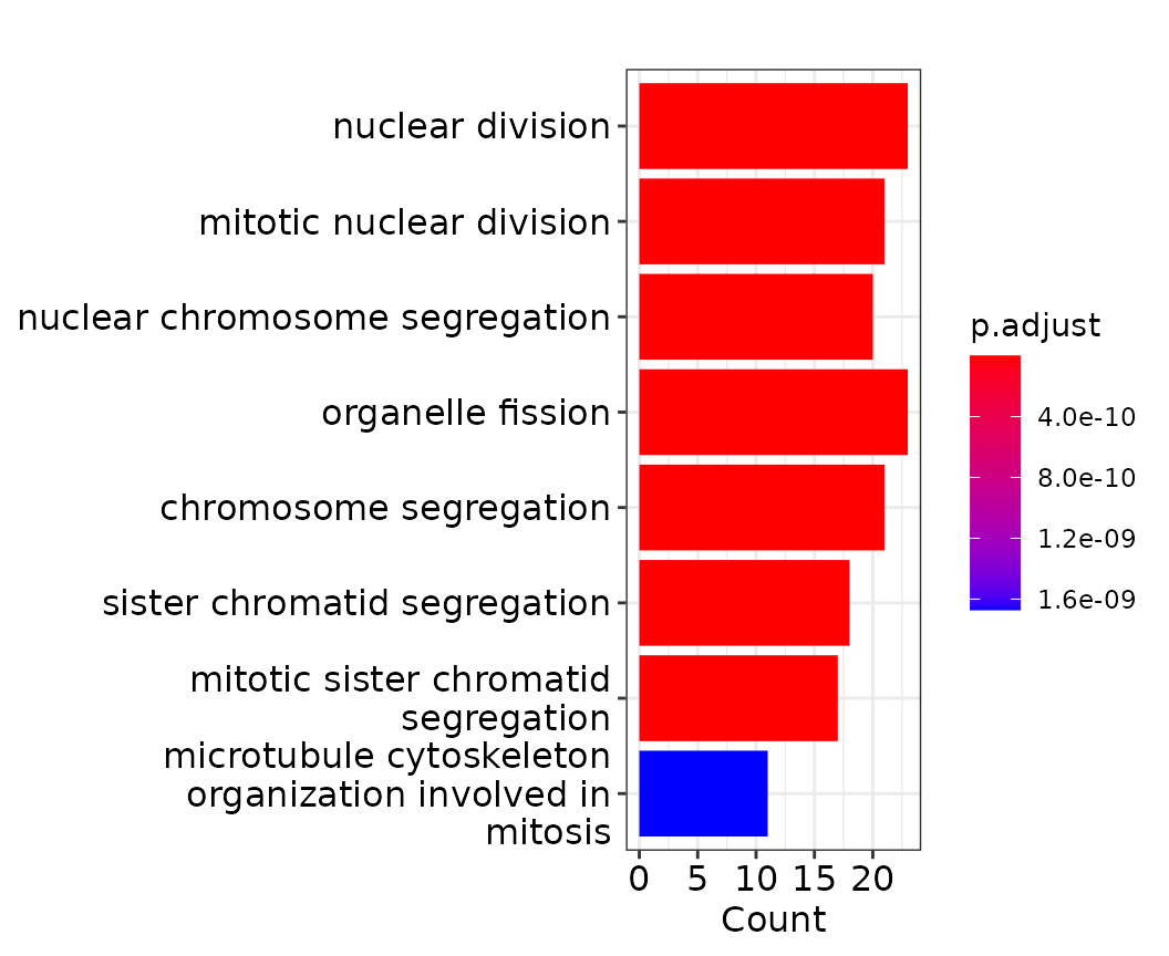
ego_up <- enrichGO(gene         = res_classify[res_classify$AUC>0.65 & res_classify$LFC>0,]$Gene,
                  OrgDb         = org.Hs.eg.db,
                  universe = res_classify$Gene,
                  keyType       = 'SYMBOL',
                  ont           = "BP",
                  pAdjustMethod = "BH",
                  pvalueCutoff  = 0.01,
                  qvalueCutoff  = 0.05)
barplot(ego_up)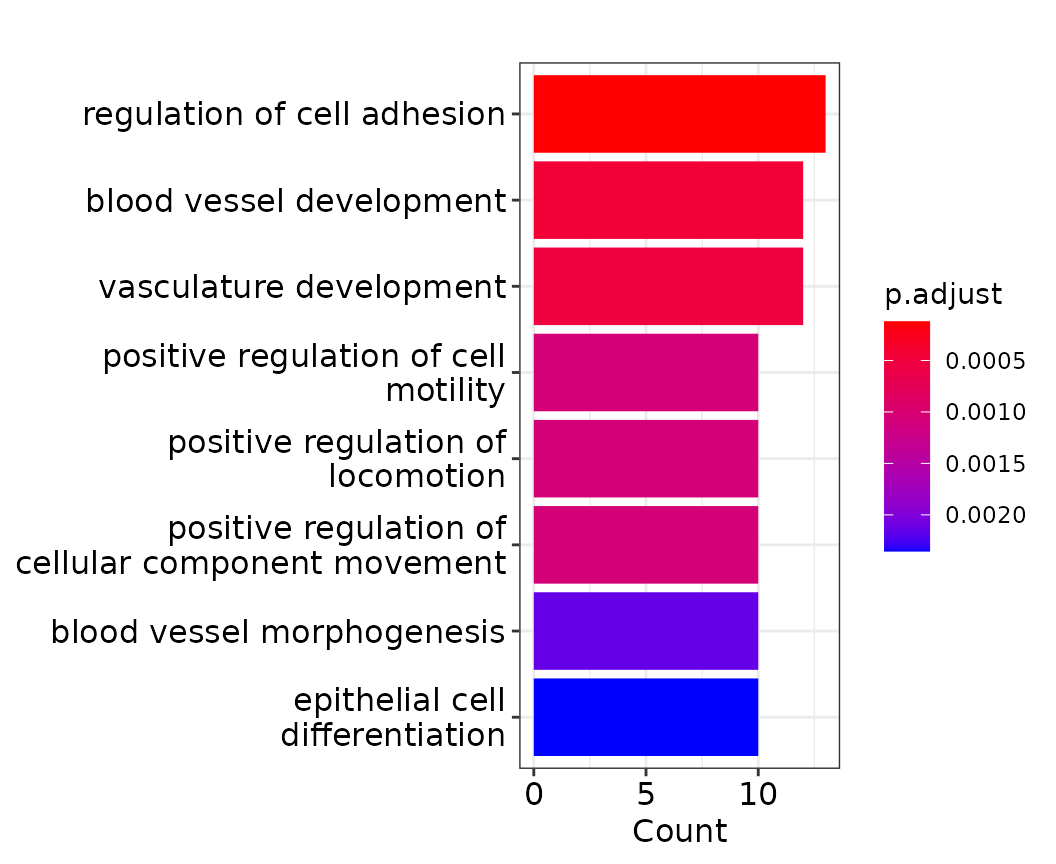
Among the negative modulators (LFC < 0), we see many genes connected to the cell cycle, which fits nicely with a [paper] reporting weaker responses to DEX during the S phase. As this effect seems to dominate the negative modulators, it might be sensible to remove the cell cycle effect from the classification results. This can be done by specifying the basefeatures parameter of the Hetseq functions. This parameter can take a vector of metadata column or gene names and will include this information in the prediction for every gene. The seurat object contains two meta data columns called cc_umap1 and cc_umap2. These are the first and second umap coordinates of a UMAP based solely on cell cycle genes. For the purpose of this demonstration, we skip this UMAP calculation (if you are interested, check the original code for our paper [here]).
res_classify_cc <- HetseqClassify(data, trajectories, score.name = "dex.percent.new", basefeatures = c("cc_umap1", "cc_umap2"), num_cores = 16)
 Low High
 263  262
PlotClassify(res_classify_cc, highlights=c("ZFP36L1", "TRAM1", "ACTN4", "SRGN", "G6PD"))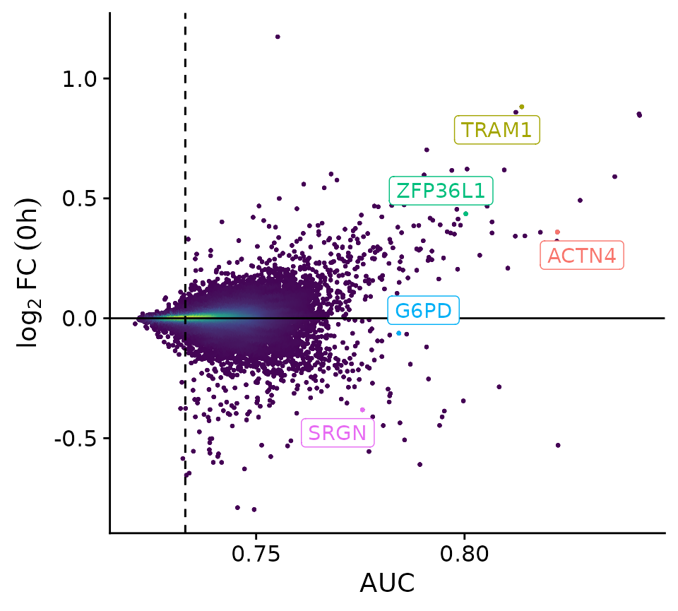
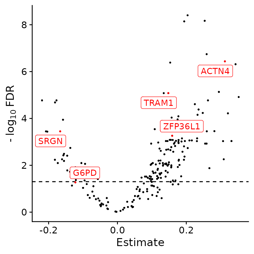
This new analysis now shows a set of genes whose AUC was calculated including the cell cycle information. Among many newly identified factors, we find several genes like [ZFP36L1], [TRAM1] and [ACTN4], who are known positive modulators as well as [SRGN] and [G6PD] who are involved in a range of drug resistances and DEX resistance, respectively.
While the classifier returns an extensive list of possible gene candidates, the DoubleML approach uses Causal Inference to identify truly causal factors and estimates their effect on the outcome. This approach is inherently more strict and runs for a significantly longer time. We strongly encourage to increase the number of cores or only use the DoubleML approach to confirm a limited set of genes. For the purpose of this vignette, we only run the DoubleML approach on 200 genes.
g_conf <- res_classify_cc[res_classify_cc$AUC>0.77,]$Gene

res_doubleml_cc <- HetseqDoubleML(data, trajectories, score.name = "dex.percent.new", genes = g_conf, basefeatures = c("cc_umap1", "cc_umap2"), num_cores = 32)
 Low High
 263  262
[1] "Iterations done"
PlotDoubleML(res_doubleml_cc, highlights=c("ZFP36L1", "TRAM1", "ACTN4", "SRGN", "G6PD"), highlights.color = rep("red", 5), density.color = FALSE)