One of the main applications of metabolic RNA labeling is to model the kinetics of RNA expression levels 12. The most natural and widely used model is to describe the change of RNA levels \(a(t)\) at time \(t\) is by the differential equation:
\[ \frac{da}{dt}=\sigma - \delta \cdot a(t) \] Here \(\sigma\) is the net synthesis rate of RNA and \(\delta\) is the degradation rate. This differential equation can be solved analytically (see e.g. [1]). Based on this, there are several ways implemented in grandR to estimate both \(\sigma\) and \(\delta\). Here, we will see how to fit this model using non-linear least squares (NLLS) regression on the estimated new and old RNA levels [2].
To perform an analysis of the RNA dynamics for data from 3, we first load the grandR package and then read the GRAND-SLAM output table directly from zenodo. All code from this vignette runs within <3 minutes on a modern laptop (Ryzen Pro 7, 1TB Ram).
suppressPackageStartupMessages({
    library(grandR)
    library(ggplot2)
    library(patchwork)
options(timeout = 600)
})
sars <- ReadGRAND("https://zenodo.org/record/5834034/files/sars.tsv.gz",
                  design=c(Design$Condition,Design$dur.4sU,Design$Replicate))
Warning: Duplicate gene symbols (n=17, e.g. TXNRD3NB,SDHD,HIST1H3D,LYNX1,MATR3,PDE11A)
present, making unique!Refer to the Loading data and working
with grandR objects vignette to learn more about how to load data.
Note that sample metadata has been automatically extracted from the
sample names via the design parameter given to
ReadGRAND:
Coldata(sars) Name Condition Replicate duration.4sU duration.4sU.original no4sU
Mock.no4sU.A Mock.no4sU.A Mock A 0 no4sU TRUE
Mock.1h.A Mock.1h.A Mock A 1 1h FALSE
Mock.2h.A Mock.2h.A Mock A 2 2h FALSE
Mock.2h.B Mock.2h.B Mock B 2 2h FALSE
Mock.3h.A Mock.3h.A Mock A 3 3h FALSE
Mock.4h.A Mock.4h.A Mock A 4 4h FALSE
SARS.no4sU.A SARS.no4sU.A SARS A 0 no4sU TRUE
SARS.1h.A SARS.1h.A SARS A 1 1h FALSE
SARS.2h.A SARS.2h.A SARS A 2 2h FALSE
SARS.2h.B SARS.2h.B SARS B 2 2h FALSE
SARS.3h.A SARS.3h.A SARS A 3 3h FALSE
SARS.4h.A SARS.4h.A SARS A 4 4h FALSEBy default GRAND-SLAM will report data on all genes (with at least
one mapped read), and ReadGRAND will read all these genes
from the output:
sarsgrandR:
Read from https://zenodo.org/record/5834034/files/sars
19659 genes, 12 samples/cells
Available data slots: count,ntr,alpha,beta
Available analyses:
Available plots:
Default data slot: countThus, we filter to only include genes that have at least 100 reads in at least 6 samples:
sars <- FilterGenes(sars,minval = 100, mincol = 6)
# as 100 reads and half of the sample is the default, this is identical to sars <- FilterGenes(sars)
sars
grandR:
Read from https://zenodo.org/record/5834034/files/sars
9162 genes, 12 samples/cells
Available data slots: count,ntr,alpha,beta
Available analyses:
Available plots:
Default data slot: countThe actual data is available in so-called “data slots”.
ReadGRAND adds the read counts, new to total RNA ratios
(NTRs) and information on the NTR posterior distribution
(alpha,beta).
As a quick quality check, we can inspect a principal component analysis of all samples involved:
PlotPCA(sars)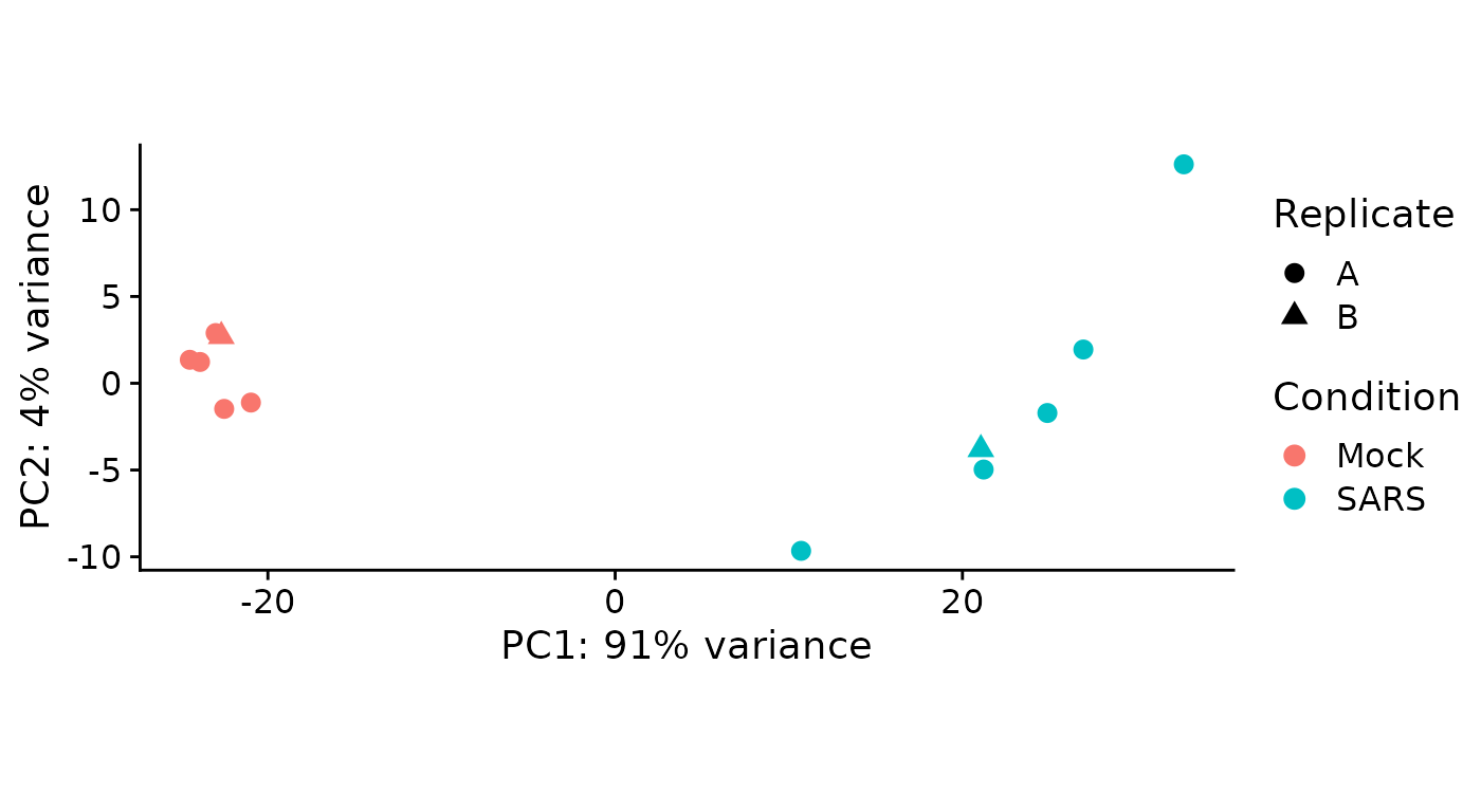
The samples are colored according to the Condition
annotation (see above in the Coldata table). Condition has
a special meaning in grandR, not only for PlotPCA, but also
for other analyses (see below). The Condition can be set
conveniently using the Condition function. For more
information, see the Loading data
vignette. For PlotPCA, the visual attributes can be
adapted via a parameter (this is the mapping parameter to ggplot, and,
thus, all names from the Coldata table can be used in expressions):
PlotPCA(sars,aest=aes(color=duration.4sU.original,shape=Condition))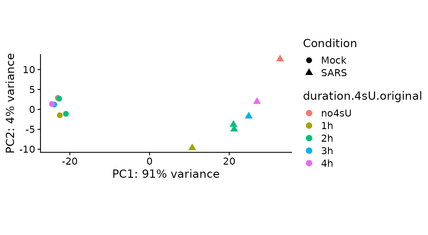 There are no obvious problems with the samples, even though the virus
infected 3hpi sample is the top-most whereas the other virus infected
samples are ordered along infection time from bottom to top.
There are no obvious problems with the samples, even though the virus
infected 3hpi sample is the top-most whereas the other virus infected
samples are ordered along infection time from bottom to top.
For the NLLS approach it is important to normalize data:
sars<-Normalize(sars)
sars
grandR:
Read from https://zenodo.org/record/5834034/files/sars
9162 genes, 12 samples/cells
Available data slots: count,ntr,alpha,beta,norm
Available analyses:
Available plots:
Default data slot: normMake sure that the normalization you use here is appropriate. Calling
Normalize will add an additional slot which is set to be
the default slot.
Before we conduct any kinetic modeling, we inspect the 4sU dropout plots:
Plot4sUDropoutRankAll(subset(sars,Condition=="Mock"))$Mock.1h.A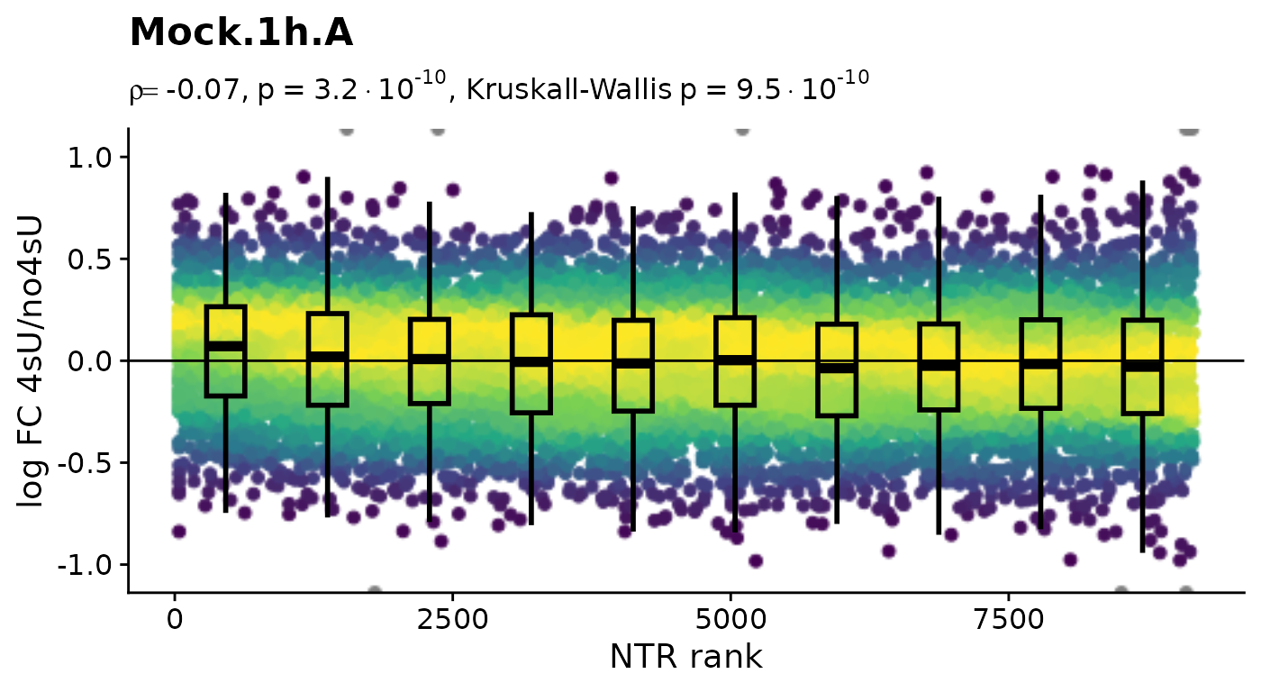
$Mock.2h.A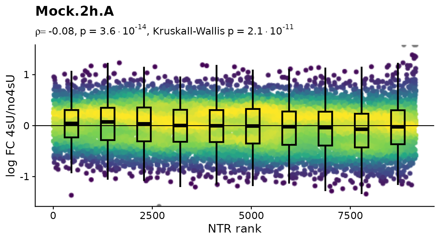
$Mock.2h.B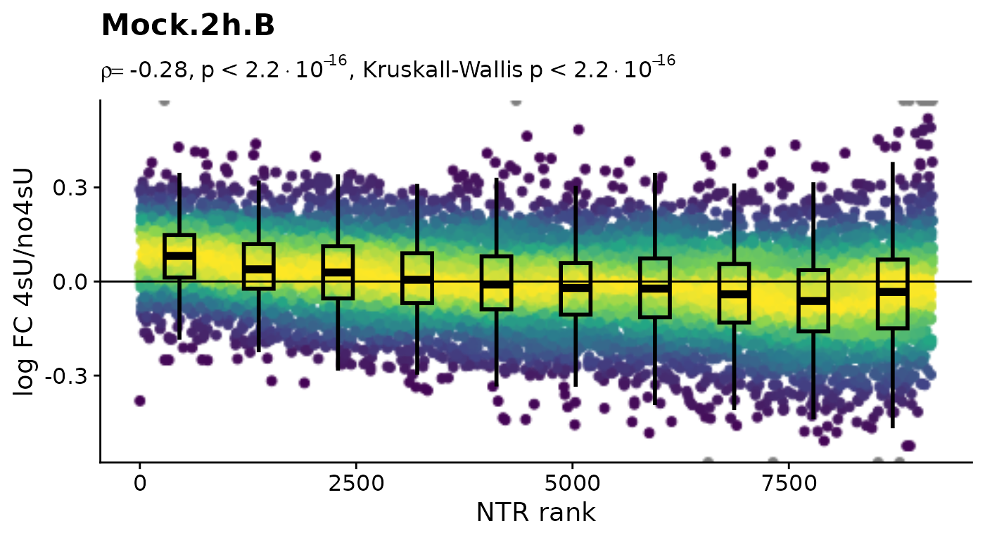
$Mock.3h.A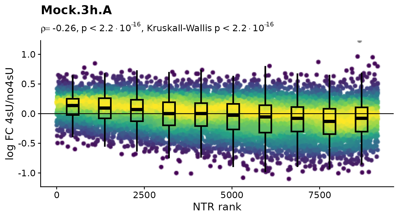
$Mock.4h.A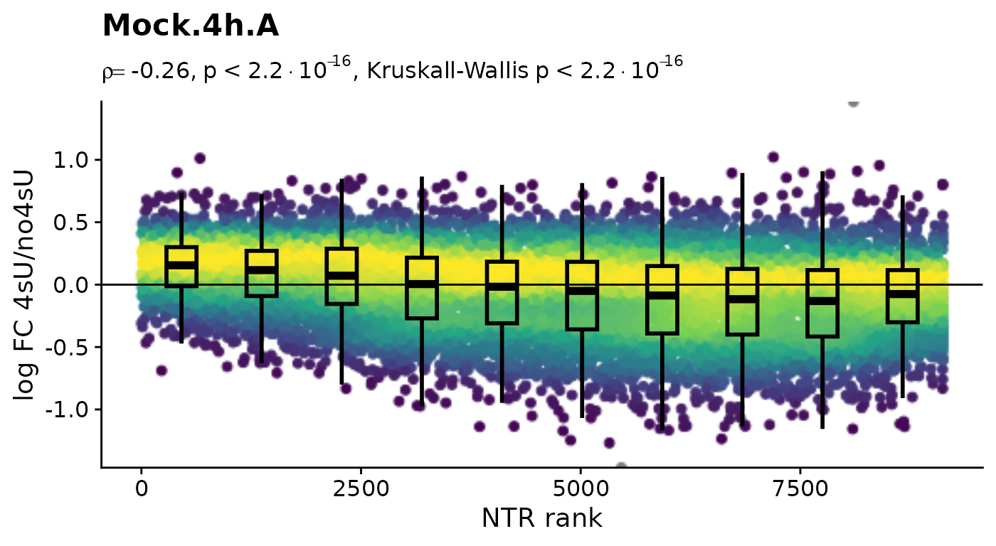 4sU labeling can have impact on transcription before cell viability
suffers. Such an effect would be observable in these plots by a
substantial negative correlation, i.e. genes with high NTR (which are to
the right), should tend to be downregulated in the 4sU labeled sample vs
an equivalent 4sU naive sample. It is important that these analyses are
only done by comparing biologically equivalent samples (and not on the
SARS infected samples here, as the no4sU sample is from 3h post
infection, and all others are later). Here, there are such effects, but
they are not very strong.
4sU labeling can have impact on transcription before cell viability
suffers. Such an effect would be observable in these plots by a
substantial negative correlation, i.e. genes with high NTR (which are to
the right), should tend to be downregulated in the 4sU labeled sample vs
an equivalent 4sU naive sample. It is important that these analyses are
only done by comparing biologically equivalent samples (and not on the
SARS infected samples here, as the no4sU sample is from 3h post
infection, and all others are later). Here, there are such effects, but
they are not very strong.
Before we estimate kinetic parameters globally, we inspect an example:
PlotGeneProgressiveTimecourse(sars,"SRSF6")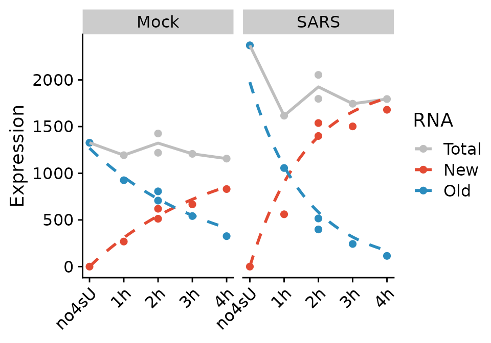
The curves represent the fitted model for this gene. The kinetic modeling by default makes the assumption of steady state gene expression, i.e. that as much RNA is transcribed per time unit as it is degraded. In mathematical terms, it is \[ \frac{da}{dt}=\sigma - \delta \cdot a(t) \Leftrightarrow a(t)=\frac{\sigma}{\delta} \] For the virus infected samples (“SARS”), this is not the case. So we specify an additional parameter:
PlotGeneProgressiveTimecourse(sars,"SRSF6",steady.state=list(Mock=TRUE,SARS=FALSE))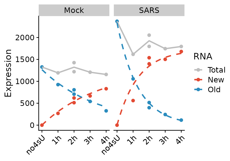
Note that the fit actually changed. Now we are ready to fit the model
for each gene. For that, we set SetParallel(cores = 2)
which will set the number of worker threads to 2 (which is the maximal
number of cores for vignettes on CRAN). Omit the cores = 2
parameter for auto-detection (“number of cores”-2). We also specify the
same steady.state parameter to
FitKinetics:
SetParallel(cores = 2) # increase on your system, or omit the cores = 2 for automatic detectionNULL
sars<-FitKinetics(sars,name = "kinetics",steady.state=list(Mock=TRUE,SARS=FALSE))FitKinetics added its result table to the grandR
object:
sarsgrandR:
Read from https://zenodo.org/record/5834034/files/sars
9162 genes, 12 samples/cells
Available data slots: count,ntr,alpha,beta,norm
Available analyses: kinetics.Mock,kinetics.SARS
Available plots:
Default data slot: normNote that there are apparently now two analyses tables. We can get
more information using the Analyses function:
Analyses(sars,description = TRUE)$kinetics.Mock
[1] "Synthesis" "Half-life"
$kinetics.SARS
[1] "Synthesis" "Half-life"This tells us that there are indeed two analysis tables, each having
a Synthesis and a Half-life column. We can retrieve the analysis results
using the GetAnalysisTable function:
df<-GetAnalysisTable(sars)
head(df)
Gene Symbol Length Type kinetics.Mock.Synthesis
MIB2 ENSG00000197530 MIB2 4247 Cellular 11.44548
OSBPL9 ENSG00000117859 OSBPL9 4520 Cellular 33.88277
BTF3L4 ENSG00000134717 BTF3L4 4703 Cellular 75.16929
ZFYVE9 ENSG00000157077 ZFYVE9 5194 Cellular 22.06668
PRPF38A ENSG00000134748 PRPF38A 5274 Cellular 84.46720
AHCYL1 ENSG00000168710 AHCYL1 4313 Cellular 33.58576
kinetics.Mock.Half-life kinetics.SARS.Synthesis kinetics.SARS.Half-life
MIB2 6.685331 37.37293 4.6532263
OSBPL9 8.936141 100.12116 2.0838946
BTF3L4 4.453564 98.62337 2.0688530
ZFYVE9 5.129308 49.96790 2.2536813
PRPF38A 2.891519 204.62499 0.9362758
AHCYL1 13.390102 106.41401 1.9559446See the Working
with data matrices and analysis results vignette for more
information how to retrieve data from a grandR object. We can use the
PlotScatter function to compare half-lives from Mock and
SARS:
PlotScatter(sars,x=`kinetics.Mock.Half-life`,y=`kinetics.SARS.Half-life`,log=TRUE)+geom_abline()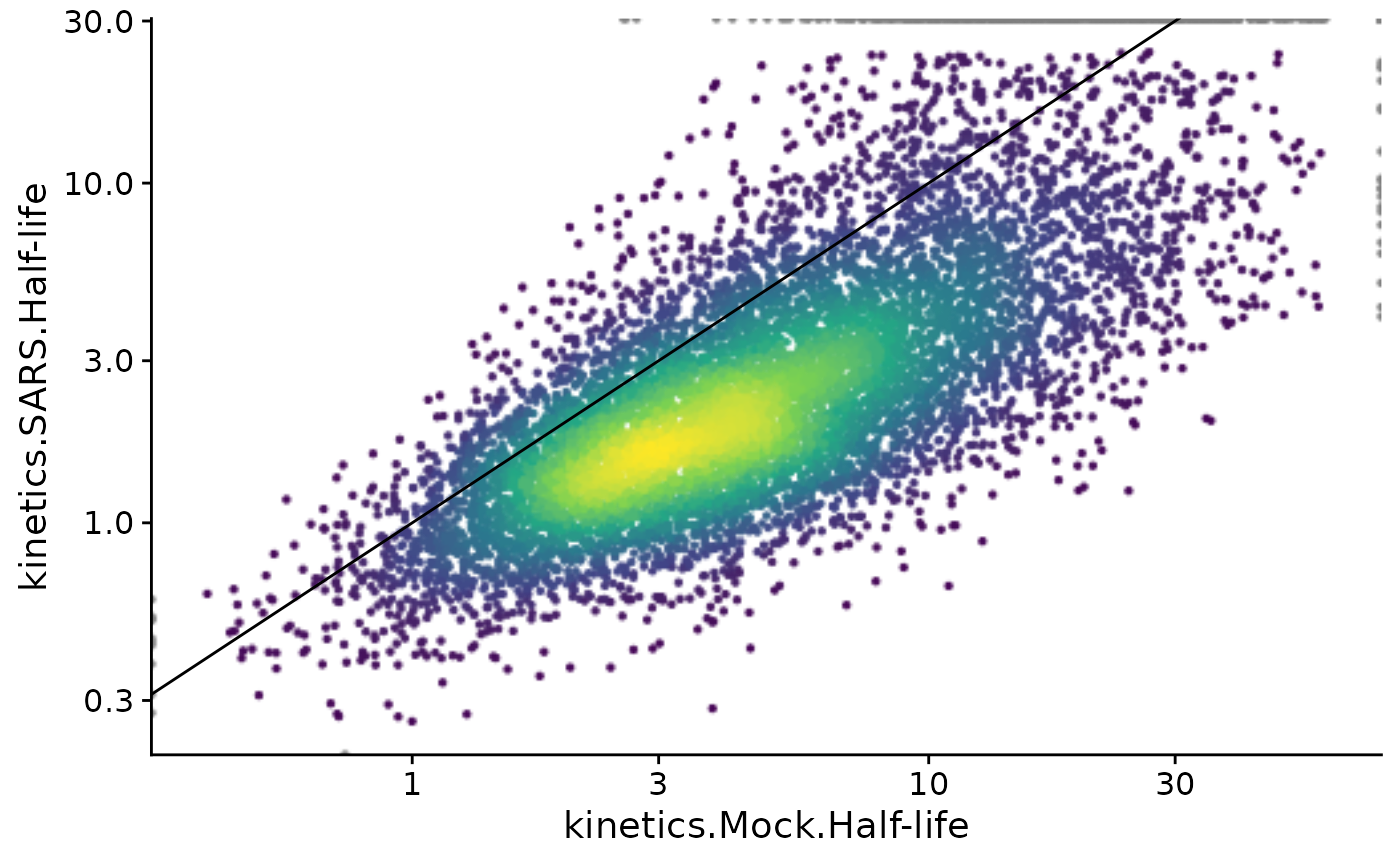
For more on PlotScatter, see the Plotting vignette. The FitKinetics
function actually computes much more information per gene. To see this,
let’s fit a single gene:
List of 2
 $ Mock:List of 14
  ..$ data       :'data.frame': 12 obs. of  10 variables:
  .. ..$ Name                 : Factor w/ 6 levels "Mock.no4sU.A",..: 1 2 3 4 5 6 1 2 3 4 ...
  .. ..$ Condition            : Factor w/ 1 level "Mock": 1 1 1 1 1 1 1 1 1 1 ...
  .. ..$ Replicate            : Factor w/ 2 levels "A","B": 1 1 1 2 1 1 1 1 1 2 ...
  .. ..$ duration.4sU         : num [1:12] 0 1 2 2 3 4 0 1 2 2 ...
  .. ..$ duration.4sU.original: Factor w/ 5 levels "no4sU","1h","2h",..: 1 2 3 3 4 5 1 2 3 3 ...
  .. ..$ no4sU                : logi [1:12] TRUE FALSE FALSE FALSE FALSE FALSE ...
  .. ..$ Value                : num [1:12] 1327 925 707 806 541 ...
  .. ..$ use                  : logi [1:12] TRUE TRUE TRUE TRUE TRUE TRUE ...
  .. ..$ time                 : num [1:12] 0 1 2 2 3 4 0 1 2 2 ...
  .. ..$ Type                 : chr [1:12] "Old" "Old" "Old" "Old" ...
  .. ..- attr(*, "vars")= chr "Condition"
  ..$ residuals  :'data.frame': 12 obs. of  4 variables:
  .. ..$ Name    : chr [1:12] "Mock.no4sU.A" "Mock.1h.A" "Mock.2h.A" "Mock.2h.B" ...
  .. ..$ Type    : chr [1:12] "old" "old" "old" "old" ...
  .. ..$ Absolute: num [1:12] 58.33 -34.12 -18.08 80.84 -6.97 ...
  .. ..$ Relative: num [1:12] 0.046 -0.0356 -0.0249 0.1115 -0.0127 ...
  ..$ Synthesis  : num 355
  ..$ Degradation: num 0.28
  ..$ Half-life  : num 2.48
  ..$ conf.lower : Named num [1:3] 315.653 0.252 2.261
  .. ..- attr(*, "names")= chr [1:3] "Synthesis" "Degradation" "Half-life"
  ..$ conf.upper : Named num [1:3] 393.591 0.307 2.745
  .. ..- attr(*, "names")= chr [1:3] "Synthesis" "Degradation" "Half-life"
  ..$ f0         : num 1269
  ..$ logLik     :Class 'logLik' : -64 (df=3)
  ..$ rmse       : num 51
  ..$ rmse.new   : num 44.6
  ..$ rmse.old   : num 56.7
  ..$ total      : num 7531
  ..$ type       : chr "equi"
 $ SARS:List of 14
  ..$ data       :'data.frame': 12 obs. of  10 variables:
  .. ..$ Name                 : Factor w/ 6 levels "SARS.no4sU.A",..: 1 2 3 4 5 6 1 2 3 4 ...
  .. ..$ Condition            : Factor w/ 1 level "SARS": 1 1 1 1 1 1 1 1 1 1 ...
  .. ..$ Replicate            : Factor w/ 2 levels "A","B": 1 1 1 2 1 1 1 1 1 2 ...
  .. ..$ duration.4sU         : num [1:12] 0 1 2 2 3 4 0 1 2 2 ...
  .. ..$ duration.4sU.original: Factor w/ 5 levels "no4sU","1h","2h",..: 1 2 3 3 4 5 1 2 3 3 ...
  .. ..$ no4sU                : logi [1:12] TRUE FALSE FALSE FALSE FALSE FALSE ...
  .. ..$ Value                : num [1:12] 2370 1056 398 516 243 ...
  .. ..$ use                  : logi [1:12] TRUE TRUE TRUE TRUE TRUE TRUE ...
  .. ..$ time                 : num [1:12] 0 1 2 2 3 4 0 1 2 2 ...
  .. ..$ Type                 : chr [1:12] "Old" "Old" "Old" "Old" ...
  .. ..- attr(*, "vars")= chr "Condition"
  ..$ residuals  :'data.frame': 12 obs. of  4 variables:
  .. ..$ Name    : chr [1:12] "SARS.no4sU.A" "SARS.1h.A" "SARS.2h.A" "SARS.2h.B" ...
  .. ..$ Type    : chr [1:12] "old" "old" "old" "old" ...
  .. ..$ Absolute: num [1:12] 32.09 -28.65 -105.27 12.31 9.13 ...
  .. ..$ Relative: num [1:12] 0.0137 -0.0264 -0.2091 0.0245 0.0391 ...
  ..$ Synthesis  : num 1318
  ..$ Degradation: num 0.768
  ..$ Half-life  : num 0.903
  ..$ conf.lower : Named num [1:3] 1073.242 0.593 0.736
  .. ..- attr(*, "names")= chr [1:3] "Synthesis" "Degradation" "Half-life"
  ..$ conf.upper : Named num [1:3] 1563.227 0.942 1.168
  .. ..- attr(*, "names")= chr [1:3] "Synthesis" "Degradation" "Half-life"
  ..$ f0         : num 2338
  ..$ logLik     :Class 'logLik' : -75 (df=4)
  ..$ rmse       : num 124
  ..$ rmse.new   : num 169
  ..$ rmse.old   : num 46.9
  ..$ total      : num 11378
  ..$ type       : chr "non.equi"
To add additional statistics to the analysis table, we use the
return.fields and return.extra parameters:
# let's perform analyses on fewer genes, it's faster
small <- FilterGenes(sars,use=1:100)
small<-FitKinetics(small,name = "with.loglik",
                   steady.state=list(Mock=TRUE,SARS=FALSE),
                   return.fields=c("Synthesis","Half-life","logLik"))
Analyses(small,description = TRUE)
$kinetics.Mock
[1] "Synthesis" "Half-life"
$kinetics.SARS
[1] "Synthesis" "Half-life"
$with.loglik.Mock
[1] "Synthesis" "Half-life" "logLik"
$with.loglik.SARS
[1] "Synthesis" "Half-life" "logLik" The logLik field could in principle be used to perform likelihood
ratio test for significant changes in the kinetics between two or among
more conditions. For values that are not directly returned fields we use
the return.extra parameter:
small<-FitKinetics(small,name = "with.loglik",
                   steady.state=list(Mock=TRUE,SARS=FALSE),
                   return.extra=function(d) c(
                       lower=d$conf.lower["Half-life"],
                       upper=d$conf.upper["Half-life"]
                       ))
Analyses(small,description = TRUE)
$kinetics.Mock
[1] "Synthesis" "Half-life"
$kinetics.SARS
[1] "Synthesis" "Half-life"
$with.loglik.Mock
[1] "Synthesis" "Half-life" "logLik" "lower.Half-life" "upper.Half-life"
$with.loglik.SARS
[1] "Synthesis" "Half-life" "logLik" "lower.Half-life" "upper.Half-life"Here, not also that the analysis table were already present, and it just added the additional columns (in fact it replaced all columns except for logLik, as this was not part of the returned analysis table).
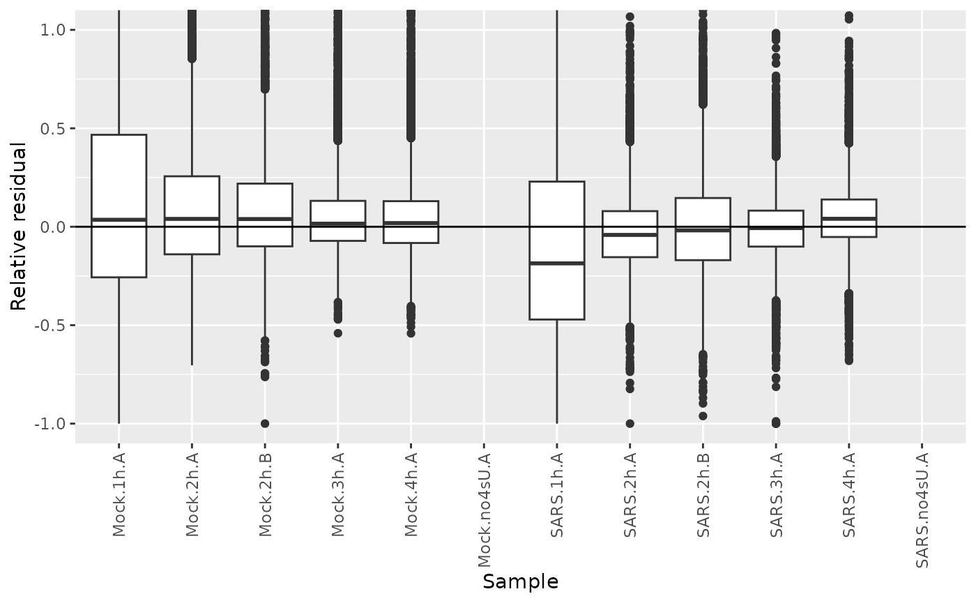
We could also extract the relative residuals of new RNA from the model fit:
sars<-FitKinetics(sars,"kinetics",steady.state=list(Mock=TRUE,SARS=FALSE),return.extra = function(s) setNames(s$residuals$Relative,paste0("Residuals.",s$residuals$Name))[s$residuals$Type=="new"])Let’s plot their distributions:
df <- GetAnalysisTable(sars,columns = "Residuals",gene.info = FALSE,prefix.by.analysis = FALSE)
df <- reshape2::melt(df,variable.name = "Sample",value.name = "Relative residual",id.vars = c())
df$Sample=gsub("Residuals.","",df$Sample)
ggplot(df,aes(Sample,`Relative residual`))+
  geom_hline(yintercept = 0)+
  geom_boxplot()+
  RotatateAxisLabels()+
  coord_cartesian(ylim=c(-1,1))
Warning:
[1m
[22mRemoved 18324 rows containing non-finite outside the scale range
(`stat_boxplot()`).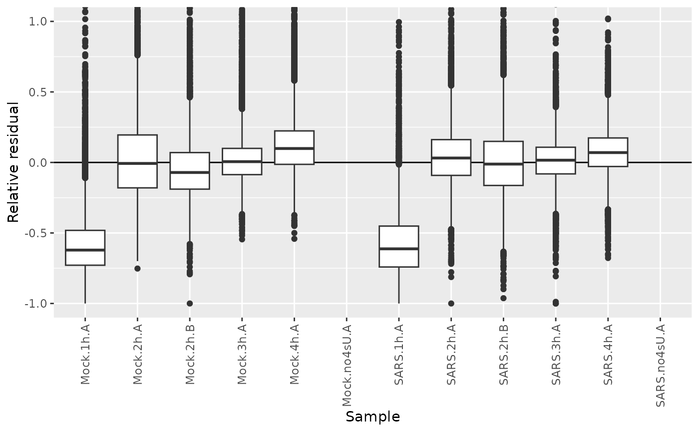
We see that the residuals from the 1h timepoints are systematically below zero. A canonical example of this is SMAD3:
PlotGeneProgressiveTimecourse(sars,"SMAD3",steady.state=list(Mock=TRUE,SARS=FALSE))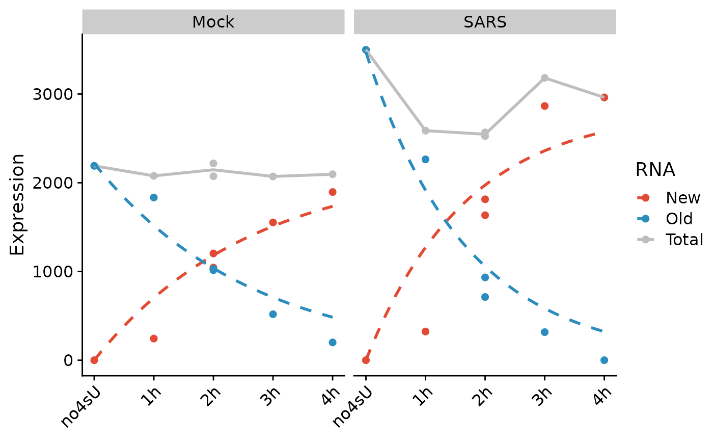 For both Mock and SARS, we see that new RNA from 1h is well below the
model fit, i.e. has negative residual. This indicates that the effective
labeling time was much lower than the nominal labeling time of 1h for
these samples, i.e. that actually, these samples should move to the
left. This can be rectified by temporal recalibration:
For both Mock and SARS, we see that new RNA from 1h is well below the
model fit, i.e. has negative residual. This indicates that the effective
labeling time was much lower than the nominal labeling time of 1h for
these samples, i.e. that actually, these samples should move to the
left. This can be rectified by temporal recalibration:
#sars <- CalibrateEffectiveLabelingTimeKineticFit(sars,steady.state=list(Mock=TRUE,SARS=FALSE))
# this takes a long time, we just use the optimized timepoint directly; feel free to uncomment and compare!
Coldata(sars,"calibrated_time") <- c(0.0000000,0.2857464,1.6275374,1.4987246,2.5506585,4.0000000,0.0000000,0.3842279,2.0826150,1.8797744,2.9423108,4.0000000)
This adds an additional column to the Coldata metadata
table:
Coldata(sars) Name Condition Replicate duration.4sU duration.4sU.original no4sU
Mock.no4sU.A Mock.no4sU.A Mock A 0 no4sU TRUE
Mock.1h.A Mock.1h.A Mock A 1 1h FALSE
Mock.2h.A Mock.2h.A Mock A 2 2h FALSE
Mock.2h.B Mock.2h.B Mock B 2 2h FALSE
Mock.3h.A Mock.3h.A Mock A 3 3h FALSE
Mock.4h.A Mock.4h.A Mock A 4 4h FALSE
SARS.no4sU.A SARS.no4sU.A SARS A 0 no4sU TRUE
SARS.1h.A SARS.1h.A SARS A 1 1h FALSE
SARS.2h.A SARS.2h.A SARS A 2 2h FALSE
SARS.2h.B SARS.2h.B SARS B 2 2h FALSE
SARS.3h.A SARS.3h.A SARS A 3 3h FALSE
SARS.4h.A SARS.4h.A SARS A 4 4h FALSE
calibrated_time
Mock.no4sU.A 0.0000000
Mock.1h.A 0.2857464
Mock.2h.A 1.6275374
Mock.2h.B 1.4987246
Mock.3h.A 2.5506585
Mock.4h.A 4.0000000
SARS.no4sU.A 0.0000000
SARS.1h.A 0.3842279
SARS.2h.A 2.0826150
SARS.2h.B 1.8797744
SARS.3h.A 2.9423108
SARS.4h.A 4.0000000This recalibrated time can now be used to plot fitted models:
PlotGeneProgressiveTimecourse(sars,"SMAD3",steady.state=list(Mock=TRUE,SARS=FALSE),
                 time = "calibrated_time",exact.tics = FALSE)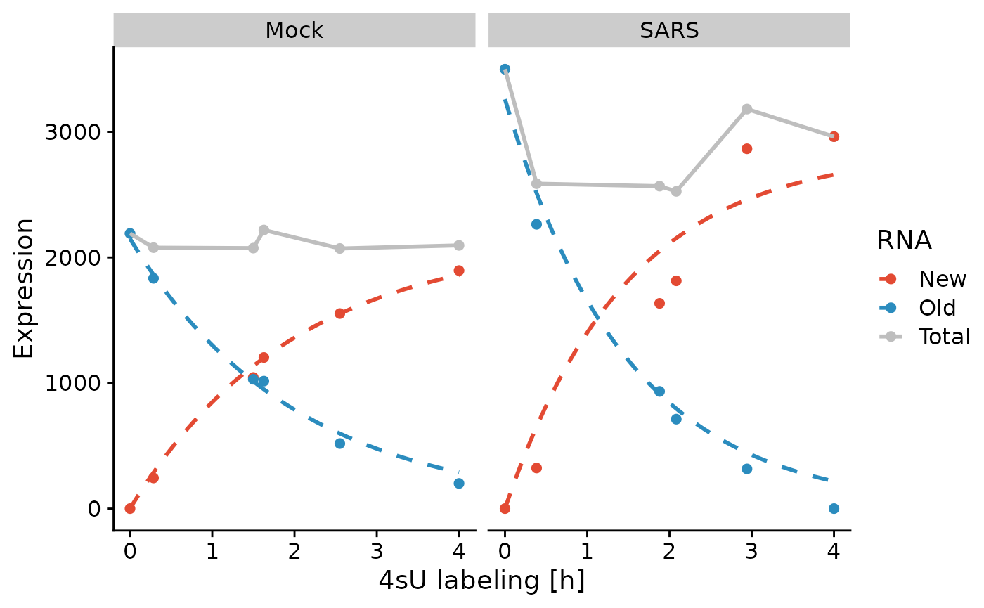
… and also to fit the model to all genes:
sars<-FitKinetics(sars,"corrected",time = "calibrated_time",steady.state=list(Mock=TRUE,SARS=FALSE),return.extra = function(s) setNames(s$residuals$Relative,paste0("Residuals.",s$residuals$Name))[s$residuals$Type=="new"])This indeed corrected the residuals:
df <- GetAnalysisTable(sars,analyses = "corrected", columns = "Residuals",gene.info = FALSE,prefix.by.analysis = FALSE)
df <- reshape2::melt(df,variable.name = "Sample",value.name = "Relative residual",id.vars = c())
df$Sample=gsub("Residuals.","",df$Sample)
ggplot(df,aes(Sample,`Relative residual`))+
  geom_boxplot()+
  RotatateAxisLabels()+
  geom_hline(yintercept = 0)+
  coord_cartesian(ylim=c(-1,1))
Warning:
[1m
[22mRemoved 18324 rows containing non-finite outside the scale range
(`stat_boxplot()`).