Here, we will show a basic example of how to correct 4sU induced dropout in a SLAM-seq data set.
We used the progressive 4sU labeling data from (paper) with labeling times from 15 min to 120 min.
At first, we load the grandR package, read in the GRAND-SLAM output and only retain genes with at least 200 reads in half of the samples.
library(grandR)
library(ggplot2)
options(timeout = 600)

r <- ReadGRAND("https://zenodo.org/record/7753473/files/nih_kinetics_rescued.tsv.gz",design=c(Design$dur.4sU,Design$Replicate))
r <- FilterGenes(r,minval = 200)
Now, we can check if we observe any dropout effects in our data set, e.g. the 120 min labeling sample.
For this, we create a dropout plot, showing us the log2 fold change for all genes between the 120 min labeling sample vs. a 4sU naïve sample.
Plot4sUDropoutRank(r,"120min.A",ylim=c(-0.5,0.5),title=NULL,size=0.6,label.corr = FALSE,invert.ranks=TRUE)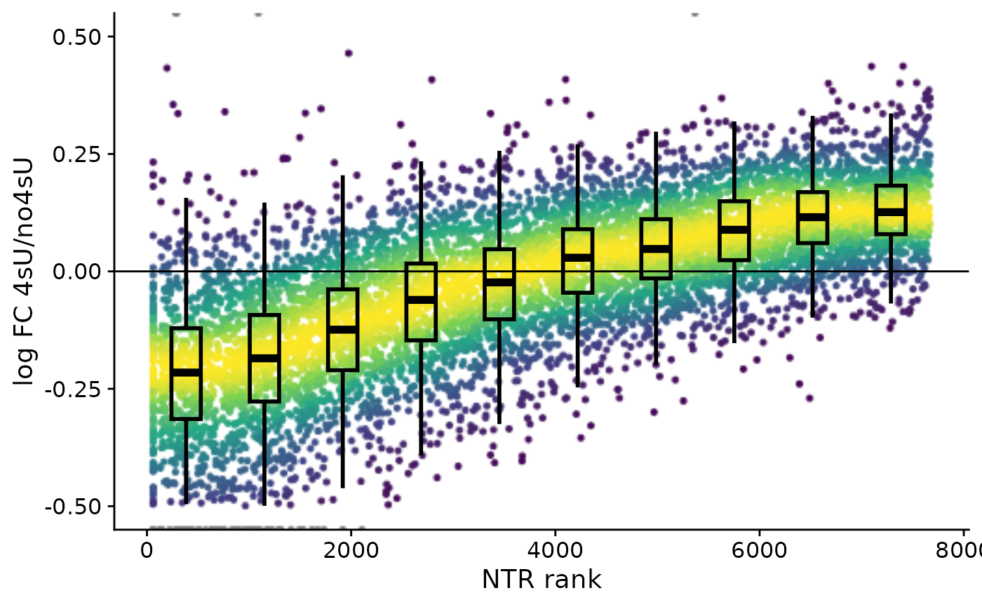
Additionally, with the Scatter plot, we can compare both replicates and confirm that the dropout effects are consistent among both replicates.
co=GetContrasts(r,contrast=c("duration.4sU.original","no4sU"),group="Replicate",no4sU=TRUE)
r=LFC(r,contrasts=co)
PlotScatter(r,`total.120min vs no4sU.A.LFC`,`total.120min vs no4sU.B.LFC`,lim=c(-1,1),correlation=FormatCorrelation(method="spearman"),xlab=bquote(log[2]~"FC 2h vs 0h (Rep. A)"),ylab=bquote(log[2]~"FC 2h vs 0h (Rep. B)"))
4sU dropout plots give a good impression about such an effect, but we can also quantify the dropout per sample.
For this, we compute a summary of the statistics in our data set and plot the dropout rate over time and as we can see, the dropout rates increase consistently in both replicates for longer labeling times.
stat.r=ComputeSummaryStatistics(r,coldata=TRUE)

ggplot(stat.r,aes(duration.4sU,`4sU dropout`,group=Replicate))+
  coord_cartesian(ylim=c(0,0.4))+
  geom_point(position=position_dodge(width=8))+
  cowplot::theme_cowplot()+
  xlab("4sU labeling [min]")+
  ylab("4sU dropout")+
  scale_x_continuous(breaks=c(0,15,30,60,90,120))+
  scale_y_continuous(labels = scales::label_percent(1),breaks=c(0,0.2,0.4))+
  RotatateAxisLabels()
Now that we’ve checked our data for 4sU dropout, we can use grandR to correct for this:
rc=Correct4sUDropoutHLFactor(r)Looking at the dropout plot for the corrected data set, we do not observe dropout effects anymore:
Plot4sUDropoutRank(rc,"120min.A",ylim=c(-0.5,0.5),title=NULL,size=0.6,label.corr = FALSE,invert.ranks=TRUE)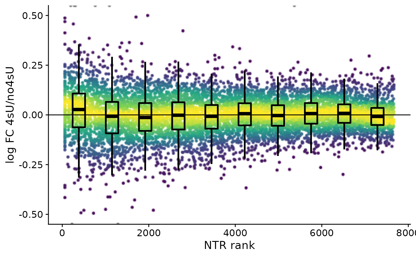
Maybe more importantly, we need to check whether 4sU induced effects are removed. For that we again compare the replicates and observe, that the correlation is gone now (indicating that any factor that still plays a role is less relevant than the differences between replicates):
rc=LFC(rc,contrasts=co)
PlotScatter(rc,`total.120min vs no4sU.A.LFC`,`total.120min vs no4sU.B.LFC`,lim=c(-1,1),correlation=FormatCorrelation(method="spearman"),xlab=bquote(log[2]~"FC 2h vs 0h (Rep. A)"),ylab=bquote(log[2]~"FC 2h vs 0h (Rep. B)"))+scale_x_continuous(breaks=c(-1,0,1))+scale_y_continuous(breaks=c(-1,0,1))