Working with data matrices and analysis results

This vignette will show the most suitable commands to retrieve data from a grandR object in different scenarios.

Throughout this vignette, we will be using the GRAND-SLAM processed SLAM-seq data set from Finkel et al. 2021 [3]. The data set contains time series (progressive labeling) samples from a human epithelial cell line (Calu3 cells); half of the samples were infected with SARS-CoV-2 for different periods of time. For more on these initial commands see the “Loading data” vignette.

suppressPackageStartupMessages({
    library(grandR)
    library(ggplot2)
    library(patchwork)
})

sars <- ReadGRAND("https://zenodo.org/record/5834034/files/sars.tsv.gz",
                  design=c("Condition",Design$dur.4sU,Design$Replicate),
                  classify.genes = ClassifyGenes(name.unknown = "Viral"))

Warning: Duplicate gene symbols (n=17, e.g. RABGEF1,TMSB15B,SCO2,KBTBD11-OT1,STPG4,COG8)
present, making unique!

sars <- FilterGenes(sars) 

Data slots

Data is organized in an grandR object in so-called slots:

Slots(sars)

[1] "count" "ntr"   "alpha" "beta" 

To learn about metadata, see the loading data vignette. After loading GRAND-SLAM analysis results, the default slots are “count” (read counts), “ntr” (the new-to-total RNA ratio) and “alpha” and “beta” (the parameters for the Beta approximation of the NTR posterior distribution). Each of these slots contains a gene x columns (columns are either samples or cells, depending on whether your data is bulk or single cell data) matrix of numeric values.

There is also a default slot, which is used by many functions as default parameter.

DefaultSlot(sars)

[1] "count"

New slots are added by specific grandR functions such as Normalize or NormalizeTPM, which, by default, also change the default slot. The default slot can also be set manually:

sars <- Normalize(sars)
DefaultSlot(sars)

[1] "norm"

DefaultSlot(sars)<-"count"
DefaultSlot(sars)

[1] "count"

sars <- NormalizeTPM(sars,set.to.default = FALSE)
DefaultSlot(sars)

[1] "count"

DefaultSlot(sars)<-"norm"

There are also other grandR functions that add additional slots, but do not update the DefaultSlot automatically:

sars <- ComputeNtrCI(sars)
DefaultSlot(sars)

[1] "norm"

Slots(sars)

[1] "count" "ntr"   "alpha" "beta"  "norm"  "tpm"   "lower" "upper"

Analyses

In addition to data slots, there is an additional kind of data that is part of a grandR object: analyses.

Analyses(sars)

NULL

After loading data there are no analyses, but such data are added e.g. by performing modeling of progressive labeling time courses or analyzing differential gene expression (see the vignettes Kinetic modeling and Differential expression for more on these):

SetParallel(cores = 2)  # increase 2 on your system, or omit the cores = 2 for automatic detection
sars <- FitKinetics(sars,name="kinetics",steady.state=c(Mock=TRUE,SARS=FALSE))
sars <- LFC(sars,contrasts=GetContrasts(sars,contrast = c("duration.4sU.original","no4sU"),
                                        group = "Condition",no4sU=TRUE))
Analyses(sars)

 [1] "kinetics.Mock"          "kinetics.SARS"          "total.1h vs no4sU.Mock"
 [4] "total.2h vs no4sU.Mock" "total.3h vs no4sU.Mock" "total.4h vs no4sU.Mock"
 [7] "total.1h vs no4sU.SARS" "total.2h vs no4sU.SARS" "total.3h vs no4sU.SARS"
[10] "total.4h vs no4sU.SARS"

Both analysis methods, FitKinetics and LFC added multiple analyses: FitKinetics added an analysis for each Condition whereas LFC added an analysis for each of many pairwise comparison defined by GetContrasts (see Differential expression for details).

What is common to data slots and analyses is that both are tables with as many rows as there are genes. What is different is that the columns of data slots always correspond to the samples or cells (depending on whether data are bulk or single cell data), and the columns of analysis tables are arbitrary and depend on the kind of analysis performed.

Analysis columns can be retrieved by setting the description parameter to TRUE for Analyses:

Analyses(sars,description = TRUE)

$kinetics.Mock
[1] "Synthesis" "Half-life"

$kinetics.SARS
[1] "Synthesis" "Half-life"

$`total.1h vs no4sU.Mock`
[1] "LFC" "M"  

$`total.2h vs no4sU.Mock`
[1] "LFC" "M"  

$`total.3h vs no4sU.Mock`
[1] "LFC" "M"  

$`total.4h vs no4sU.Mock`
[1] "LFC" "M"  

$`total.1h vs no4sU.SARS`
[1] "LFC" "M"  

$`total.2h vs no4sU.SARS`
[1] "LFC" "M"  

$`total.3h vs no4sU.SARS`
[1] "LFC" "M"  

$`total.4h vs no4sU.SARS`
[1] "LFC" "M"  

We see that the FitKinetics function by default creates tables with two columns (Synthesis and Half-life) corresponding to the synthesis rate and RNA half-life for each gene, and the LFC function creates a single column called LFC corresponding to the log2 fold change for each gene.

Retrieving data from slots or analyses

There are essentially three functions you can use for retrieving slot data:

• GetTable: The swiss army knive, returns a data frame with genes as rows and columns made from potentially several slots and/or analyses; usually for all or at least a lot of genes
• GetData: Returns a data frame with the samples or cells as rows and slot data for particular genes in columns; usually for a single or at most very few genes
• GetAnalysisTable: Returns a data frame with genes as rows and columns made from potentially several analyses; usually for all or at least a lot of genes; there is (almost) no need to call this function (see below for exceptions)

GetTable

Without any other parameters GetTable returns data for all genes from the default slot:

head(GetTable(sars))

	Mock.no4sU.A	Mock.1h.A	Mock.2h.A	Mock.2h.B	Mock.3h.A	Mock.4h.A	SARS.no4sU.A	SARS.1h.A	SARS.2h.A	SARS.2h.B	SARS.3h.A	SARS.4h.A
MIB2	50.61593	138.9483	152.6633	100.2339	116.0365	127.5967	175.5632	210.7226	275.4692	190.0241	231.7082	191.9265
OSBPL9	480.85133	397.6568	386.5828	466.7414	429.5386	421.7695	476.5287	407.3970	399.1705	435.3603	340.6110	348.1020
BTF3L4	578.46777	399.6418	302.8643	545.1853	526.9991	417.5061	501.6091	431.9813	269.2322	446.9580	382.3185	398.9061
ZFYVE9	184.38660	160.7831	157.1775	158.6311	127.9964	131.8601	238.2643	193.1624	168.4001	210.5431	192.3178	203.2163
PRPF38A	357.92693	310.3179	335.6951	364.7643	329.7880	362.6913	501.6091	278.6221	309.7730	365.7740	315.1231	312.3510
AHCYL1	708.62302	569.6881	581.9262	707.7386	641.7633	653.5143	589.3907	361.7405	384.6174	410.3806	421.7089	423.3673

You can change the slot by specifying another type parameter:

head(GetTable(sars,type="count"))

	Mock.no4sU.A	Mock.1h.A	Mock.2h.A	Mock.2h.B	Mock.3h.A	Mock.4h.A	SARS.no4sU.A	SARS.1h.A	SARS.2h.A	SARS.2h.B	SARS.3h.A	SARS.4h.A
MIB2	14	420	372	230	456	419	14	180	265	213	100	102
OSBPL9	133	1202	942	1071	1688	1385	38	348	384	488	147	185
BTF3L4	160	1208	738	1251	2071	1371	40	369	259	501	165	212
ZFYVE9	51	486	383	364	503	433	19	165	162	236	83	108
PRPF38A	99	938	818	837	1296	1191	40	238	298	410	136	166
AHCYL1	196	1722	1418	1624	2522	2146	47	309	370	460	182	225

You can use multiple slots (we only show the column names instead of the head of the returned table):

colnames(GetTable(sars,type=c("norm","count")))

 [1] "Mock.no4sU.A.norm"  "Mock.1h.A.norm"     "Mock.2h.A.norm"     "Mock.2h.B.norm"    
 [5] "Mock.3h.A.norm"     "Mock.4h.A.norm"     "SARS.no4sU.A.norm"  "SARS.1h.A.norm"    
 [9] "SARS.2h.A.norm"     "SARS.2h.B.norm"     "SARS.3h.A.norm"     "SARS.4h.A.norm"    
[13] "Mock.no4sU.A.count" "Mock.1h.A.count"    "Mock.2h.A.count"    "Mock.2h.B.count"   
[17] "Mock.3h.A.count"    "Mock.4h.A.count"    "SARS.no4sU.A.count" "SARS.1h.A.count"   
[21] "SARS.2h.A.count"    "SARS.2h.B.count"    "SARS.3h.A.count"    "SARS.4h.A.count"   

By using the mode.slot syntax (mode being either of total,new and old), you can also retrieve new RNA counts or new RNA normalized values:

head(GetTable(sars,type="new.norm"))

	Mock.no4sU.A	Mock.1h.A	Mock.2h.A	Mock.2h.B	Mock.3h.A	Mock.4h.A	SARS.no4sU.A	SARS.1h.A	SARS.2h.A	SARS.2h.B	SARS.3h.A	SARS.4h.A
MIB2	NA	2.334332	32.10509	16.46843	40.35750	52.62088	NA	10.325408	68.12354	38.99294	110.7333	116.5570
OSBPL9	NA	17.337839	55.16537	62.35665	82.90096	109.74443	NA	49.254301	154.35924	181.37111	169.2155	224.5606
BTF3L4	NA	17.304491	69.29534	120.86759	177.28251	223.49103	NA	40.303858	101.58131	177.39764	194.9442	232.5622
ZFYVE9	NA	2.267041	27.86758	25.77755	39.24370	68.76503	NA	3.283761	56.46454	66.65795	100.9091	144.2633
PRPF38A	NA	28.735438	122.15944	133.94145	160.30993	252.36062	NA	82.304970	223.16044	235.55848	231.8361	284.3331
AHCYL1	NA	12.988889	66.68874	59.59159	88.56334	117.43653	NA	14.469619	134.00072	139.28318	214.9450	262.4454

Note that the no4sU columns only have NA values. You can change this behavior by specifying the ntr.na parameter:

head(GetTable(sars,type="new.norm",ntr.na = FALSE))

	Mock.no4sU.A	Mock.1h.A	Mock.2h.A	Mock.2h.B	Mock.3h.A	Mock.4h.A	SARS.no4sU.A	SARS.1h.A	SARS.2h.A	SARS.2h.B	SARS.3h.A	SARS.4h.A
MIB2	0	2.334332	32.10509	16.46843	40.35750	52.62088	0	10.325408	68.12354	38.99294	110.7333	116.5570
OSBPL9	0	17.337839	55.16537	62.35665	82.90096	109.74443	0	49.254301	154.35924	181.37111	169.2155	224.5606
BTF3L4	0	17.304491	69.29534	120.86759	177.28251	223.49103	0	40.303858	101.58131	177.39764	194.9442	232.5622
ZFYVE9	0	2.267041	27.86758	25.77755	39.24370	68.76503	0	3.283761	56.46454	66.65795	100.9091	144.2633
PRPF38A	0	28.735438	122.15944	133.94145	160.30993	252.36062	0	82.304970	223.16044	235.55848	231.8361	284.3331
AHCYL1	0	12.988889	66.68874	59.59159	88.56334	117.43653	0	14.469619	134.00072	139.28318	214.9450	262.4454

GetTable can also be used to retrieve analysis results:

head(GetTable(sars,type="kinetics"))

	kinetics.Mock.Synthesis	kinetics.Mock.Half-life	kinetics.SARS.Synthesis	kinetics.SARS.Half-life
MIB2	11.44548	6.685331	37.37293	4.6532263
OSBPL9	33.88277	8.936141	100.12116	2.0838946
BTF3L4	75.16929	4.453564	98.62337	2.0688530
ZFYVE9	22.06668	5.129308	49.96790	2.2536813
PRPF38A	84.46720	2.891519	204.62499	0.9362758
AHCYL1	33.58576	13.390102	106.41401	1.9559446

Note that you do not have to specify the full name (it actually is a regular expression that is matched against each analysis name).

It is also easily possible to only retrieve data for specific columns (i.e., samples or cells) by using the columns parameter. Note that you can use names from the Coldata table to construct a logical vector over the columns; using a character vector (to specify names) or a numeric vector (to specify positions) also works:

head(GetTable(sars,columns=duration.4sU>=2 & Condition=="Mock"))

	Mock.2h.A	Mock.2h.B	Mock.3h.A	Mock.4h.A
MIB2	152.6633	100.2339	116.0365	127.5967
OSBPL9	386.5828	466.7414	429.5386	421.7695
BTF3L4	302.8643	545.1853	526.9991	417.5061
ZFYVE9	157.1775	158.6311	127.9964	131.8601
PRPF38A	335.6951	364.7643	329.7880	362.6913
AHCYL1	581.9262	707.7386	641.7633	653.5143

head(GetTable(sars,columns=c("Mock.no4sU.A","SARS.no4sU.A")))

	Mock.no4sU.A	SARS.no4sU.A
MIB2	50.61593	175.5632
OSBPL9	480.85133	476.5287
BTF3L4	578.46777	501.6091
ZFYVE9	184.38660	238.2643
PRPF38A	357.92693	501.6091
AHCYL1	708.62302	589.3907

head(GetTable(sars,columns=4:6))

	Mock.2h.B	Mock.3h.A	Mock.4h.A
MIB2	100.2339	116.0365	127.5967
OSBPL9	466.7414	429.5386	421.7695
BTF3L4	545.1853	526.9991	417.5061
ZFYVE9	158.6311	127.9964	131.8601
PRPF38A	364.7643	329.7880	362.6913
AHCYL1	707.7386	641.7633	653.5143

It is furthermore possible to only fetch data for specific genes, e.g. viral genes using the genes parameter. It is either a logical vector, a numeric vector, or gene names/symbols:

GetTable(sars,genes=GeneInfo(sars,"Type")=="Viral")

	Mock.no4sU.A	Mock.1h.A	Mock.2h.A	Mock.2h.B	Mock.3h.A	Mock.4h.A	SARS.no4sU.A	SARS.1h.A	SARS.2h.A	SARS.2h.B	SARS.3h.A	SARS.4h.A
ORF3a	705.0076	567.3723	807.2277	577.8703	574.3298	570.3785	2083095	218342.6	606628.0	784826.2	1246796.1	1507097.3
E	423.0046	343.4008	471.1222	336.4373	326.7344	328.5843	1169941	121044.9	328393.6	467000.7	759154.7	950348.6
M	1974.0213	1531.0781	2081.0633	1585.4390	1504.9121	1485.1768	5267423	552293.4	1647309.2	1968405.8	3039142.1	3810695.3
ORF6	473.6205	428.4240	536.7838	410.0874	402.3108	387.3580	1775044	166706.2	506668.0	551540.9	788120.5	985535.1
ORF7a	1142.4738	864.1262	1186.4236	892.5176	855.0058	836.5349	3535316	313785.9	872093.0	1217287.1	1703059.6	2043968.5
ORF7b	719.4693	502.1989	677.1356	503.7844	468.7264	470.1893	1860092	190325.8	489639.8	712069.3	1086081.0	1301399.1
ORF8	1822.1735	1316.0390	1731.4151	1287.3521	1222.9637	1209.8847	4927896	456242.5	1341787.8	1795438.4	2533144.8	3068775.1
N	8843.3260	7476.4119	10056.0785	7570.2752	7072.8831	7040.9623	25288888	2505283.4	9100887.5	9091438.6	12024874.9	14564147.9
ORF10	1663.0948	1425.5436	1843.8606	1420.2710	1323.2233	1297.5884	5242405	522616.6	1723751.4	1748268.8	2504647.0	3128464.3
ORF1ab	1659.4794	1462.5964	1874.2291	1472.1311	1389.1300	1366.1069	4954281	628565.6	1404586.5	2085797.9	2881680.2	3340669.1
S	965.3181	836.9982	1090.3934	828.4551	779.1750	766.4938	3405763	335616.7	811972.1	1160304.8	1635192.3	1968855.6

GetTable(sars,genes=1:3)

	Mock.no4sU.A	Mock.1h.A	Mock.2h.A	Mock.2h.B	Mock.3h.A	Mock.4h.A	SARS.no4sU.A	SARS.1h.A	SARS.2h.A	SARS.2h.B	SARS.3h.A	SARS.4h.A
MIB2	50.61593	138.9483	152.6633	100.2339	116.0365	127.5967	175.5632	210.7226	275.4692	190.0241	231.7082	191.9265
OSBPL9	480.85133	397.6568	386.5828	466.7414	429.5386	421.7695	476.5287	407.3970	399.1705	435.3603	340.6110	348.1020
BTF3L4	578.46777	399.6418	302.8643	545.1853	526.9991	417.5061	501.6091	431.9813	269.2322	446.9580	382.3185	398.9061

GetTable(sars,genes="MYC")

	Mock.no4sU.A	Mock.1h.A	Mock.2h.A	Mock.2h.B	Mock.3h.A	Mock.4h.A	SARS.no4sU.A	SARS.1h.A	SARS.2h.A	SARS.2h.B	SARS.3h.A	SARS.4h.A
MYC	1547.401	1577.394	2542.747	1927.106	2126.318	2047.333	3436.023	2231.318	5206.889	3753.198	4386.235	4340.926

Sometimes, it makes sense to add the GeneInfo table (for more on gene metadata, see the loading data vignette):

df <- GetTable(sars,type="norm",gene.info = TRUE)
head(df)

	Gene	Symbol	Length	Type	Mock.no4sU.A	Mock.1h.A	Mock.2h.A	Mock.2h.B	Mock.3h.A	Mock.4h.A	SARS.no4sU.A	SARS.1h.A	SARS.2h.A	SARS.2h.B	SARS.3h.A	SARS.4h.A
MIB2	ENSG00000197530	MIB2	4247	Cellular	50.61593	138.9483	152.6633	100.2339	116.0365	127.5967	175.5632	210.7226	275.4692	190.0241	231.7082	191.9265
OSBPL9	ENSG00000117859	OSBPL9	4520	Cellular	480.85133	397.6568	386.5828	466.7414	429.5386	421.7695	476.5287	407.3970	399.1705	435.3603	340.6110	348.1020
BTF3L4	ENSG00000134717	BTF3L4	4703	Cellular	578.46777	399.6418	302.8643	545.1853	526.9991	417.5061	501.6091	431.9813	269.2322	446.9580	382.3185	398.9061
ZFYVE9	ENSG00000157077	ZFYVE9	5194	Cellular	184.38660	160.7831	157.1775	158.6311	127.9964	131.8601	238.2643	193.1624	168.4001	210.5431	192.3178	203.2163
PRPF38A	ENSG00000134748	PRPF38A	5274	Cellular	357.92693	310.3179	335.6951	364.7643	329.7880	362.6913	501.6091	278.6221	309.7730	365.7740	315.1231	312.3510
AHCYL1	ENSG00000168710	AHCYL1	4313	Cellular	708.62302	569.6881	581.9262	707.7386	641.7633	653.5143	589.3907	361.7405	384.6174	410.3806	421.7089	423.3673

ggplot(df,aes(`SARS.4h.A`,`SARS.no4sU.A`,color=Type))+
  geom_point()+
  scale_x_log10()+
  scale_y_log10()+
  geom_abline()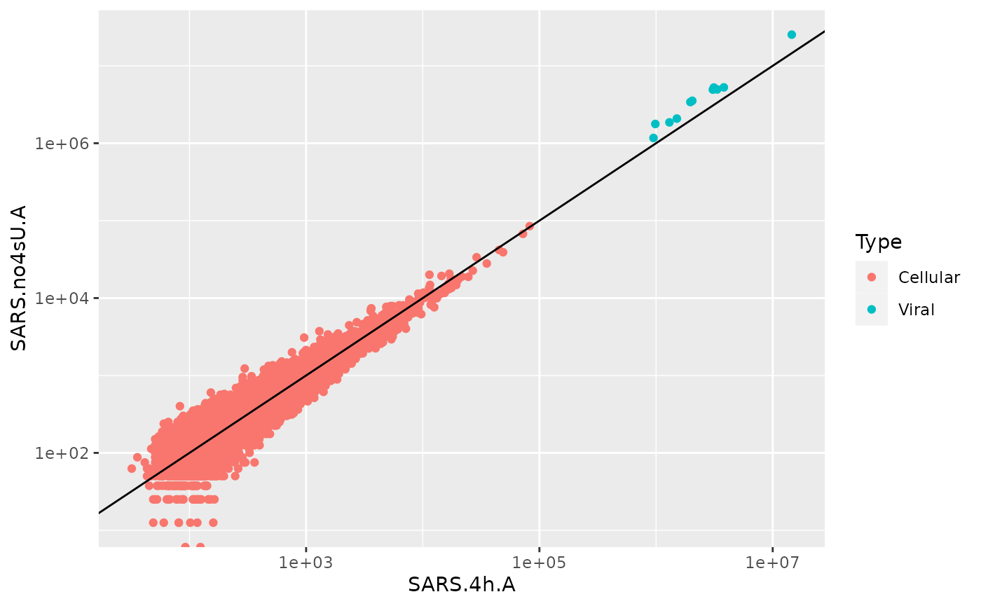

Finally, it is also straight-forward to get summarized values across samples or cells from the same Condition:

head(GetTable(sars,summarize = TRUE))

	Mock	SARS
MIB2	127.0957	219.9701
OSBPL9	420.4578	386.1282
BTF3L4	438.4393	385.8792
ZFYVE9	147.2896	193.5279
PRPF38A	340.6513	316.3286
AHCYL1	630.9261	400.3629

This is accomplished by a “summarize matrix”:

smat <- GetSummarizeMatrix(sars)
smat

             Mock SARS
Mock.no4sU.A  0.0  0.0
Mock.1h.A     0.2  0.0
Mock.2h.A     0.2  0.0
Mock.2h.B     0.2  0.0
Mock.3h.A     0.2  0.0
Mock.4h.A     0.2  0.0
SARS.no4sU.A  0.0  0.0
SARS.1h.A     0.0  0.2
SARS.2h.A     0.0  0.2
SARS.2h.B     0.0  0.2
SARS.3h.A     0.0  0.2
SARS.4h.A     0.0  0.2

Instead of specifying TRUE for the summarize parameter, you can also specify such a matrix:

head(GetTable(sars,summarize = smat))  

	Mock	SARS
MIB2	127.0957	219.9701
OSBPL9	420.4578	386.1282
BTF3L4	438.4393	385.8792
ZFYVE9	147.2896	193.5279
PRPF38A	340.6513	316.3286
AHCYL1	630.9261	400.3629

For summarization, the summarize matrix is matrix-multiplied with the raw matrix. GetSummarizeMatrix will generate a matrix with columns corresponding to Conditions:

Condition(sars)

 [1] Mock Mock Mock Mock Mock Mock SARS SARS SARS SARS SARS SARS
Levels: Mock SARS

By default, no4sU columns are removed (i.e. zero in the matrix), but the no4sU parameter can change this:

GetSummarizeMatrix(sars,no4sU = TRUE)

                  Mock      SARS
Mock.no4sU.A 0.1666667 0.0000000
Mock.1h.A    0.1666667 0.0000000
Mock.2h.A    0.1666667 0.0000000
Mock.2h.B    0.1666667 0.0000000
Mock.3h.A    0.1666667 0.0000000
Mock.4h.A    0.1666667 0.0000000
SARS.no4sU.A 0.0000000 0.1666667
SARS.1h.A    0.0000000 0.1666667
SARS.2h.A    0.0000000 0.1666667
SARS.2h.B    0.0000000 0.1666667
SARS.3h.A    0.0000000 0.1666667
SARS.4h.A    0.0000000 0.1666667

It is also possible to focus on specific columns (samples or cells) only:

GetSummarizeMatrix(sars,columns = duration.4sU<4)

             Mock SARS
Mock.no4sU.A 0.00 0.00
Mock.1h.A    0.25 0.00
Mock.2h.A    0.25 0.00
Mock.2h.B    0.25 0.00
Mock.3h.A    0.25 0.00
Mock.4h.A    0.00 0.00
SARS.no4sU.A 0.00 0.00
SARS.1h.A    0.00 0.25
SARS.2h.A    0.00 0.25
SARS.2h.B    0.00 0.25
SARS.3h.A    0.00 0.25
SARS.4h.A    0.00 0.00

The default behavior is to compute the average, this can be change to computing sums:

GetSummarizeMatrix(sars,average = FALSE)

             Mock SARS
Mock.no4sU.A    0    0
Mock.1h.A       1    0
Mock.2h.A       1    0
Mock.2h.B       1    0
Mock.3h.A       1    0
Mock.4h.A       1    0
SARS.no4sU.A    0    0
SARS.1h.A       0    1
SARS.2h.A       0    1
SARS.2h.B       0    1
SARS.3h.A       0    1
SARS.4h.A       0    1

As a final example, to get averaged normalized expression values for the 2h timepoint only:

head(GetTable(sars,summarize = GetSummarizeMatrix(sars,columns=duration.4sU==2)))

	Mock	SARS
MIB2	126.4486	232.7467
OSBPL9	426.6621	417.2654
BTF3L4	424.0248	358.0951
ZFYVE9	157.9043	189.4716
PRPF38A	350.2297	337.7735
AHCYL1	644.8324	397.4990

GetData

GetData is the little cousin of GetTable: It returns a data frame with the samples or cells as rows and slot data for either a single gene or very few genes:

GetData(sars,genes="MYC")

	Name	Condition	Replicate	duration.4sU	duration.4sU.original	no4sU	Value
Mock.no4sU.A	Mock.no4sU.A	Mock	A	0	no4sU	TRUE	1547.401
Mock.1h.A	Mock.1h.A	Mock	A	1	1h	FALSE	1577.394
Mock.2h.A	Mock.2h.A	Mock	A	2	2h	FALSE	2542.747
Mock.2h.B	Mock.2h.B	Mock	B	2	2h	FALSE	1927.106
Mock.3h.A	Mock.3h.A	Mock	A	3	3h	FALSE	2126.318
Mock.4h.A	Mock.4h.A	Mock	A	4	4h	FALSE	2047.333
SARS.no4sU.A	SARS.no4sU.A	SARS	A	0	no4sU	TRUE	3436.023
SARS.1h.A	SARS.1h.A	SARS	A	1	1h	FALSE	2231.318
SARS.2h.A	SARS.2h.A	SARS	A	2	2h	FALSE	5206.889
SARS.2h.B	SARS.2h.B	SARS	B	2	2h	FALSE	3753.198
SARS.3h.A	SARS.3h.A	SARS	A	3	3h	FALSE	4386.235
SARS.4h.A	SARS.4h.A	SARS	A	4	4h	FALSE	4340.926

Note that by default, the Coldata table is also added (for more on column metadata, see the loading data vignette). Note that in contrast to GetTable, where you can add the GeneInfo table, i.e. gene metadata, here it is the columns metadata! This can be changed by using the coldata parameter:

GetData(sars,genes="MYC",coldata = FALSE)

	Value
Mock.no4sU.A	1547.401
Mock.1h.A	1577.394
Mock.2h.A	2542.747
Mock.2h.B	1927.106
Mock.3h.A	2126.318
Mock.4h.A	2047.333
SARS.no4sU.A	3436.023
SARS.1h.A	2231.318
SARS.2h.A	5206.889
SARS.2h.B	3753.198
SARS.3h.A	4386.235
SARS.4h.A	4340.926

It is also possible to retrieve data for multiple genes and/or multiple slots, and to restrict the columns:

# multiple genes
GetData(sars,genes=c("MYC","SRSF6"),columns=Condition=="Mock",coldata = FALSE)

	MYC	SRSF6
Mock.no4sU.A	1547.401	1326.860
Mock.1h.A	1577.394	1193.301
Mock.2h.A	2542.747	1219.665
Mock.2h.B	1927.106	1425.936
Mock.3h.A	2126.318	1207.950
Mock.4h.A	2047.333	1156.897

# multiple slots, as above, compute also for no4sU samples instead of NA
GetData(sars,mode.slot=c("new.norm","old.norm"),genes="MYC",
        columns=Condition=="Mock",coldata = FALSE, ntr.na = FALSE)

	new.norm	old.norm
Mock.no4sU.A	0.0000	1547.4013
Mock.1h.A	979.0886	598.3056
Mock.2h.A	2542.7466	0.0000
Mock.2h.B	1927.1059	0.0000
Mock.3h.A	2126.3181	0.0000
Mock.4h.A	2047.3331	0.0000

# multiple genes and slots
GetData(sars,mode.slot=c("count","norm"),genes=c("MYC","SRSF6"),
        columns=Condition=="Mock",coldata = FALSE)

	MYC.count	SRSF6.count	MYC.norm	SRSF6.norm
Mock.no4sU.A	428	367	1547.401	1326.860
Mock.1h.A	4768	3607	1577.394	1193.301
Mock.2h.A	6196	2972	2542.747	1219.665
Mock.2h.B	4422	3272	1927.106	1425.936
Mock.3h.A	8356	4747	2126.318	1207.950
Mock.4h.A	6723	3799	2047.333	1156.897

Finally, it is also possible to append multiple genes (and/or slots) not as columns, but as additional rows:

GetData(sars,genes=c("MYC","SRSF6"),columns=duration.4sU<2,by.rows = TRUE)

Name	Condition	Replicate	duration.4sU	duration.4sU.original	no4sU	Gene	Value
Mock.no4sU.A	Mock	A	0	no4sU	TRUE	MYC	1547.401
Mock.1h.A	Mock	A	1	1h	FALSE	MYC	1577.394
SARS.no4sU.A	SARS	A	0	no4sU	TRUE	MYC	3436.023
SARS.1h.A	SARS	A	1	1h	FALSE	MYC	2231.318
Mock.no4sU.A	Mock	A	0	no4sU	TRUE	SRSF6	1326.860
Mock.1h.A	Mock	A	1	1h	FALSE	SRSF6	1193.301
SARS.no4sU.A	SARS	A	0	no4sU	TRUE	SRSF6	2370.103
SARS.1h.A	SARS	A	1	1h	FALSE	SRSF6	1616.711

This can be quite helpful, as for the following example: We retrieve total, old and new RNA for SRSF6 (only replicate A), and do this by rows. This way, the data can directly be used for ggplot to plot the progressive labeling time course (note the much shorter half-life, which is the time where the new and old lines cross, for SARS as compared to Mock):

df <- GetData(sars,mode.slot=c("old.norm","new.norm","total.norm"),genes="SRSF6",
              columns=Replicate=="A",by.rows = TRUE)
ggplot(df,aes(duration.4sU,Value,color=mode.slot))+
  geom_line()+
  facet_wrap(~Condition)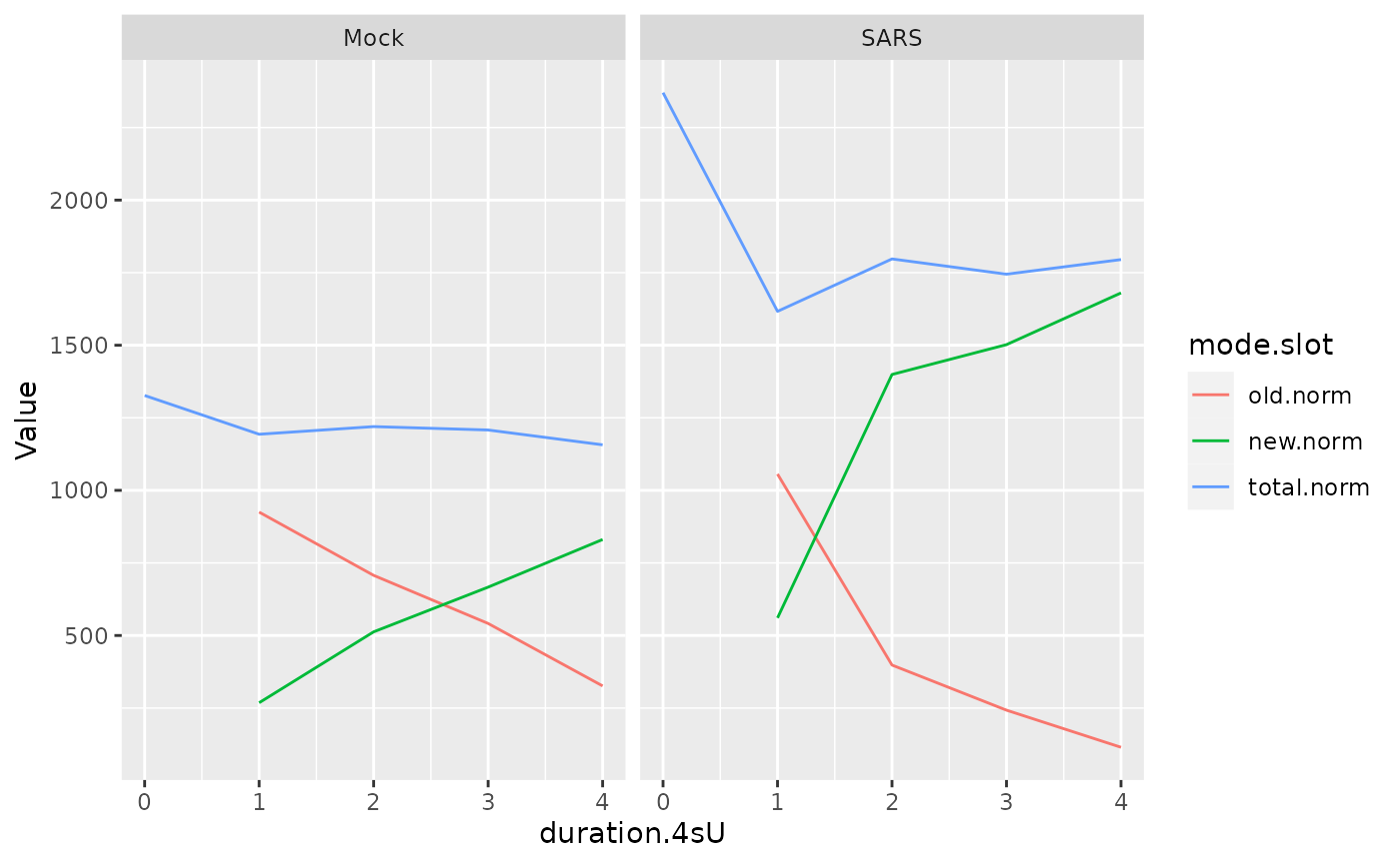

GetAnalysisTable

As indicated above, GetTable can also be used to retrieve analysis results. However, sometimes it is better to be explicit when coding analysis scripts, and you can use GetAnalysisTable instead. Furthermore, there are two additional benefits of GetAnalysisTable over GetTable: First, by default, the prefix for each column of the returned table is the analysis name, which cannot be turned off when using GetTable (also note that the GeneInfo table is added by default for GetAnalysisTable, can be turned off by setting the gene.info parameter to FALSE)

head(GetTable(sars,"kinetics.Mock"))

	kinetics.Mock.Synthesis	kinetics.Mock.Half-life
MIB2	11.44548	6.685331
OSBPL9	33.88277	8.936141
BTF3L4	75.16929	4.453564
ZFYVE9	22.06668	5.129308
PRPF38A	84.46720	2.891519
AHCYL1	33.58576	13.390102

head(GetAnalysisTable(sars,"kinetics.Mock"))

	Gene	Symbol	Length	Type	kinetics.Mock.Synthesis	kinetics.Mock.Half-life
MIB2	ENSG00000197530	MIB2	4247	Cellular	11.44548	6.685331
OSBPL9	ENSG00000117859	OSBPL9	4520	Cellular	33.88277	8.936141
BTF3L4	ENSG00000134717	BTF3L4	4703	Cellular	75.16929	4.453564
ZFYVE9	ENSG00000157077	ZFYVE9	5194	Cellular	22.06668	5.129308
PRPF38A	ENSG00000134748	PRPF38A	5274	Cellular	84.46720	2.891519
AHCYL1	ENSG00000168710	AHCYL1	4313	Cellular	33.58576	13.390102

head(GetAnalysisTable(sars,"kinetics.Mock",prefix.by.analysis = FALSE))

	Gene	Symbol	Length	Type	Synthesis	Half-life
MIB2	ENSG00000197530	MIB2	4247	Cellular	11.44548	6.685331
OSBPL9	ENSG00000117859	OSBPL9	4520	Cellular	33.88277	8.936141
BTF3L4	ENSG00000134717	BTF3L4	4703	Cellular	75.16929	4.453564
ZFYVE9	ENSG00000157077	ZFYVE9	5194	Cellular	22.06668	5.129308
PRPF38A	ENSG00000134748	PRPF38A	5274	Cellular	84.46720	2.891519
AHCYL1	ENSG00000168710	AHCYL1	4313	Cellular	33.58576	13.390102

Turning off the prefixes might sound like a minor aesthetic surgery, but is quite important in some cases. Imagine you want to fit the kinetic model (i) for the full time course (as we have already done) and (ii) after removing some time points:

restricted <- subset(sars,columns = duration.4sU!=1)
restricted <- FitKinetics(restricted,name="restricted",steady.state=c(Mock=TRUE,SARS=FALSE))

And now you want to put these analyses back into the original sars object for comparison. You can use the AddAnalysis function, but here it is important not to add the prefixes for consistency:

# we need to omit prefixes and gene info, since the analysis table to be added 
# should have columns Synthesis and Half-life only
mock.tab <- GetAnalysisTable(restricted,analyses="restricted.Mock",
                         prefix.by.analysis = FALSE,gene.info = FALSE)
sars.tab <- GetAnalysisTable(restricted,analyses="restricted.SARS",
                         prefix.by.analysis = FALSE,gene.info = FALSE)

sars <- AddAnalysis(sars,"restricted.Mock",mock.tab)
sars <- AddAnalysis(sars,"restricted.SARS",sars.tab)
Analyses(sars)

 [1] "kinetics.Mock"          "kinetics.SARS"          "total.1h vs no4sU.Mock"
 [4] "total.2h vs no4sU.Mock" "total.3h vs no4sU.Mock" "total.4h vs no4sU.Mock"
 [7] "total.1h vs no4sU.SARS" "total.2h vs no4sU.SARS" "total.3h vs no4sU.SARS"
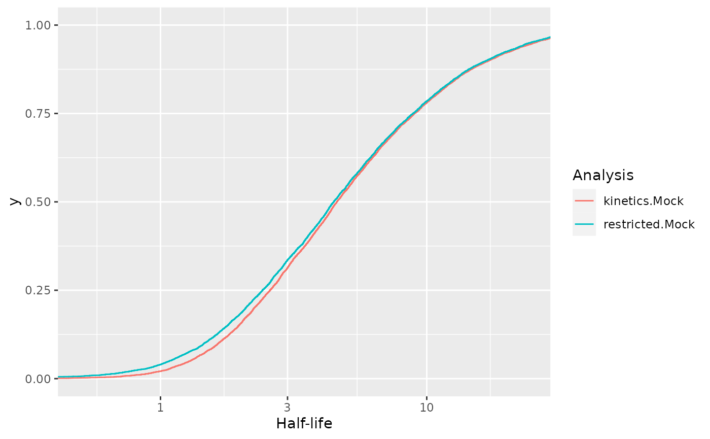
[10] "total.4h vs no4sU.SARS" "restricted.Mock"        "restricted.SARS"       

Now we want to compare the distributions of half-lives with and without removing the 1h timepoint. This can be accomplished by using the by.row parameter

df <- GetAnalysisTable(sars,c("kinetics.Mock","restricted.Mock"),
                       columns = "Half-life",by.rows = TRUE)
rbind(head(df,4),tail(df,4))

	Gene	Symbol	Length	Type	Analysis	Half-life
1	ENSG00000197530	MIB2	4247	Cellular	kinetics.Mock	6.685331
2	ENSG00000117859	OSBPL9	4520	Cellular	kinetics.Mock	8.936141
3	ENSG00000134717	BTF3L4	4703	Cellular	kinetics.Mock	4.453564
4	ENSG00000157077	ZFYVE9	5194	Cellular	kinetics.Mock	5.129308
18321	ENSG00000196924	FLNA	8486	Cellular	restricted.Mock	16.850448
18322	ENSG00000013563	DNASE1L1	3008	Cellular	restricted.Mock	9.819117
18323	ORF1ab	ORF1ab	21290	Viral	restricted.Mock	1.729493
18324	S	S	3822	Viral	restricted.Mock	1.585582

Now we can directly create an ecdf plot from this using ggplot, and we see that there are significant changes for short half-lives:

ggplot(df,aes(`Half-life`,color=Analysis))+
  stat_ecdf()+
  scale_x_log10()+
  coord_cartesian(xlim=c(0.5,24))