Loading data and working with grandR objects
Source:vignettes/web/loading-data.Rmd
loading-data.RmdgrandR is an R package for the analysis of RNA-seq experiments involving metabolic RNA labeling with nucleotide conversion, such as SLAM-seq experiments [1]. In such experiments, nucleoside analogs such as 4sU are added to living cells, which take it up and incorporate it into newly synthesized RNA. Before sequencing, 4sU is converted into a cytosin analog. Reads covering 4sU sites therefore have characteristic T-to-C mismatches after read mapping, in principle providing the opportunity to differentiate newly synthesized (during the time of labeling) from pre-existing RNA.
Confounders such as sequencing errors or reads that originate from newly synthesized RNA but, by chance, do not cover sites of 4sU incorporation (usually 20-80% of all “new reads”) can be handled using specialized methods such as GRAND-SLAM [2].
Reading in the data
Throughout this vignette, we will be using the GRAND-SLAM processed SLAM-seq data set from Finkel et al. 2021 [3]. The data set contains time series (progressive labeling) samples from a human epithelial cell line (Calu3 cells); half of the samples were infected with SARS-CoV-2 for different periods of time.
The output of GRAND-SLAM is a tsv file where rows are genes and columns are read counts and other statistics (e.g., the new-to-total RNA ratio) for all samples. The data set is available on zenodo (“https://zenodo.org/record/5834034/files/sars.tsv.gz”). We start by reading this file into R:
suppressPackageStartupMessages({
    library(grandR)
    library(ggplot2)
    library(patchwork)
    options(timeout = 600)
})
sars <- ReadGRAND("https://zenodo.org/record/5834034/files/sars.tsv.gz",
                  design=c(Design$Condition,Design$dur.4sU,Design$Replicate))
Columns(sars)
[1] "Mock.no4sU.A" "Mock.1h.A" "Mock.2h.A" "Mock.2h.B" "Mock.3h.A" "Mock.4h.A"
[7] "SARS.no4sU.A" "SARS.1h.A" "SARS.2h.A" "SARS.2h.B" "SARS.3h.A" "SARS.4h.A" When reading in the file, we have to define the design
vector. This is used to infer metadata automatically from sample names.
Here sample names consist of three parts separated by dots as shown
above (the Columns function returns the sample names or cell ids when
analyzing a single cell data set). Each part in the sample name
represents an aspect of the design. For example, the sample named
Mock.2h.A is a sample from the mock condition (i.e. not infected by
SARS-CoV-2), subjected to metabolic labeling for 2 hours, and is the
first replicate (i.e. replicate “A”). This sample name is consistent
with the three element design vector used above. It is possible to
specify other design elements (of course the samples would have to be
named accordingly). A list of reasonable options is predefined in the
list Design.
There are names (i.e. the things you specify in the design vector)
that have additional semantics. For example, for the name
duration.4sU the values are interpreted like this: 4h is
converted into the number 4, 30min into 0.5, and no4sU into 0. For more
information, see below
The design vector is mandatory. Attempting to read in the data without it results in an error:
sars <- ReadGRAND("https://zenodo.org/record/5834034/files/sars.tsv.gz")Error in read.grand.internal(prefix = prefix, design = design, slots = slots, : Design parameter is incompatible with input data: Mock.no4sU.A, Mock.1h.A, Mock.2h.A, Mock.2h.B, Mock.3h.A, Mock.4h.A, SARS.no4sU.A, SARS.1h.A, SARS.2h.A, SARS.2h.B, SARS.3h.A, SARS.4h.AAlternatively, a table containing the metadata can be specified. Make
sure that it contains a Name column matching the names in
the GRAND-SLAM output table:
metadata = data.frame(Name=c(
"Mock.no4sU.A","Mock.1h.A","Mock.2h.A","Mock.2h.B","Mock.3h.A","Mock.4h.A",
"SARS.no4sU.A","SARS.1h.A","SARS.2h.A","SARS.2h.B","SARS.3h.A","SARS.4h.A"
),Condition=rep(c("Mock","SARS"),each=6))
sars.meta <- ReadGRAND("https://zenodo.org/record/5834034/files/sars.tsv.gz",design=metadata)Warning: Duplicate gene symbols (n=17, e.g. TXNRD3NB,MATR3,SOGA3,EMG1,SPATA13,RABGEF1)
present, making unique!What is in the grandR object
ReadGRAND returns a grandR object, which contains
- metadata for genes
- metadata for samples/cells (as inferred from the sample names by the design parameter)
- all data matrices (counts, normalized counts, ntrs, etc. these types of data are called “slots”)
- analysis results
Metadata (1. and 2.) are described below. How to work with the data matrices and analysis results is described in a separate vignette.
Working with grandR objects
Here we will see how to work with grandR objects in general. A short
summmary can be displayed when printing the object, and
there are several functions to retrieve general information about the
object:
print(sars)grandR:
Read from https://zenodo.org/record/5834034/files/sars
19659 genes, 12 samples/cells
Available data slots: count,ntr,alpha,beta
Available analyses:
Available plots:
Default data slot: count
Title(sars)[1] "sars"
nrow(sars)[1] 19659
ncol(sars)[1] 12It is straight-forward to filter genes:
sars <- FilterGenes(sars)
nrow(sars)[1] 9162By default genes are retained if they have 100 read counts in at
least half of the samples (or cells). There are many options how to
filter by genes (note that FilterGenes returns a new grandR
object, and below we directly call nrow on this new object
to check how many genes are retained by filtering):
cat(sprintf("Genes with at least 1000 read counts in half of the columns: %d\n",
nrow(FilterGenes(sars,minval=1000))))Genes with at least 1000 read counts in half of the columns: 1528
cat(sprintf("Genes with at least 1000 read counts in half of the columns (retain two genes that are otherwise filtered): %d\n",
nrow(FilterGenes(sars,minval=1000,keep=c("ATF3","ZC3H12A")))))Genes with at least 1000 read counts in half of the columns (retain two genes that are otherwise filtered): 1530Keep only these two genes: 2
sars <- NormalizeTPM(sars) # compute transcript per million
cat(sprintf("Genes with at least 10 TPM in half of the columns: %d\n",
nrow(FilterGenes(sars,mode.slot="tpm",minval=10))))Genes with at least 10 TPM in half of the columns: 7795FilterGenes essentially removes rows from the data
slots. It is also possible to remove columns (i.e. samples or cells).
This is done using the subset function:
mock <- subset(sars,columns = Condition=="Mock")
mockgrandR:
Read from https://zenodo.org/record/5834034/files/sars
9162 genes, 6 samples/cells
Available data slots: count,ntr,alpha,beta,tpm
Available analyses:
Available plots:
Default data slot: tpmThe new grandR object now only has 6 columns. The
columns parameter to subset must be a logical vector, and
you can use the names of the column metadata table (see below) as
variables (i.e. the parameter here is a logical vector with all samples
being TRUE where the Condition column is equal to
“Mock”.
A closely related function is split, which returns a
list of several grandR objects, each composed of samples having the same
Condition.
split.list <- split(sars)
split.list$Mock
grandR:
Read from https://zenodo.org/record/5834034/files/sars
9162 genes, 6 samples/cells
Available data slots: count,ntr,alpha,beta,tpm
Available analyses:
Available plots:
Default data slot: tpm
$SARS
grandR:
Read from https://zenodo.org/record/5834034/files/sars
9162 genes, 6 samples/cells
Available data slots: count,ntr,alpha,beta,tpm
Available analyses:
Available plots:
Default data slot: tpm
lapply(split.list,Columns)$Mock
[1] "Mock.no4sU.A" "Mock.1h.A" "Mock.2h.A" "Mock.2h.B" "Mock.3h.A" "Mock.4h.A"
$SARS
[1] "SARS.no4sU.A" "SARS.1h.A" "SARS.2h.A" "SARS.2h.B" "SARS.3h.A" "SARS.4h.A" The inverse of split is merge:
sars.mock <- merge(split.list$SARS,split.list$Mock)
Columns(sars.mock) [1] "SARS.no4sU.A" "SARS.1h.A" "SARS.2h.A" "SARS.2h.B" "SARS.3h.A" "SARS.4h.A"
[7] "Mock.no4sU.A" "Mock.1h.A" "Mock.2h.A" "Mock.2h.B" "Mock.3h.A" "Mock.4h.A" Note that we merged such that now we have first the SARS samples and
then the Mock samples. We can reorder by slightly abusing
subset (note that we actually do not omit any columns, but
just define a different order):
 [1] "Mock.no4sU.A" "Mock.1h.A"    "Mock.2h.A"    "Mock.2h.B"    "Mock.3h.A"    "Mock.4h.A"
[7] "SARS.no4sU.A" "SARS.1h.A" "SARS.2h.A" "SARS.2h.B" "SARS.3h.A" "SARS.4h.A" Gene metadata
Here we see how to work with metadata for genes. The gene metadata
essentially is a table that can be retrieved using the
GeneInfo function:
head(GeneInfo(sars), 10) Gene Symbol Length Type
27 ENSG00000197530 MIB2 4247 Cellular
34 ENSG00000117859 OSBPL9 4520 Cellular
35 ENSG00000134717 BTF3L4 4703 Cellular
36 ENSG00000157077 ZFYVE9 5194 Cellular
37 ENSG00000134748 PRPF38A 5274 Cellular
42 ENSG00000168710 AHCYL1 4313 Cellular
44 ENSG00000117114 ADGRL2 6302 Cellular
45 ENSG00000134709 HOOK1 5857 Cellular
46 ENSG00000162599 NFIA 9487 Cellular
47 ENSG00000132849 PATJ 8505 CellularEach gene has associated gene ids and symbols. Gene ids and symbols
as well as the transcript length are part of the GRAND-SLAM output. The
Type column is inferred automatically (see below).
Genes can be identified by the Genes function:
head(Genes(sars), n=20) # retrieve the first 20 genes [1] "MIB2" "OSBPL9" "BTF3L4" "ZFYVE9" "PRPF38A" "AHCYL1" "ADGRL2"
[8] "HOOK1" "NFIA" "PATJ" "VANGL1" "GPR89B" "GPSM2" "ARHGEF10L"
[15] "TMEM50A" "TMEM57" "ZNF593" "RNF207" "ZNF362" "STX12"
head(Genes(sars,use.symbols = FALSE), n=20) # the first 20 genes, but now use the ids [1] "ENSG00000197530" "ENSG00000117859" "ENSG00000134717" "ENSG00000157077" "ENSG00000134748"
[6] "ENSG00000168710" "ENSG00000117114" "ENSG00000134709" "ENSG00000162599" "ENSG00000132849"
[11] "ENSG00000173218" "ENSG00000188092" "ENSG00000121957" "ENSG00000074964" "ENSG00000183726"
[16] "ENSG00000204178" "ENSG00000142684" "ENSG00000158286" "ENSG00000160094" "ENSG00000117758"
Genes(sars,genes = c("MYC","ORF1ab"),use.symbols = FALSE) # convert to ids[1] "ENSG00000136997" "ORF1ab"
Genes(sars,genes = "YC", regex = TRUE) # retrieve all genes matching to the regular expression YC [1] "NFYC" "MYCBP" "PYCR2" "GLYCTK" "FYCO1" "CYCS" "CYC1" "MYC" "PYCR3" "MYCBP2"
[11] "MLYCD" "PYCR1" "SYCP2" During reading the data into R using ReadGRAND, the
Type column is inferred using the
ClassifyGenes() function. By default, this will recognize
mitochondrial genes (MT prefix of the gene symbol), ERCC spike-ins, and
Ensembl gene identifiers (which it will call “cellular”). Here, we also
have the viral genes, which are not properly recognized:
table(GeneInfo(sars,"Type"))
Cellular  Unknown
    9151       11
If you want to define your own types, you can do this easily be
specifying the classify.genes parameter when read in your
data:
viral.genes <- c('ORF3a','E','M','ORF6','ORF7a','ORF7b','ORF8','N','ORF10','ORF1ab','S')
sars <- ReadGRAND("https://zenodo.org/record/5834034/files/sars.tsv.gz",
                  design=c(Design$Condition,Design$dur.4sU,Design$Replicate),
                  classify.genes = ClassifyGenes(viral=function(gene.info) gene.info$Symbol %in% viral.genes))
Warning: Duplicate gene symbols (n=17, e.g. TMSB15B,EMG1,SPATA13,SDHD,SOGA3,POLR2J2) present,
making unique!
table(GeneInfo(sars,"Type"))
   viral Cellular
      11    19648
Note that each parameter to ClassifyGenes must be named
(viral) and must be a function that takes the gene metadata
table and returns a logical vector.
The ClassifyGenes function has one additional important
parameter, which defines how “Unknown” types are supposed to be called.
For this data set, a similar behavior as above can be accomplished
by:
sars <- ReadGRAND("https://zenodo.org/record/5834034/files/sars.tsv.gz",
                  design=c(Design$Condition,Design$dur.4sU,Design$Replicate),
                  classify.genes = ClassifyGenes(name.unknown = "viral"))
table(GeneInfo(sars,"Type"))
Cellular    viral
   19648       11
It is also straight-forward to add additional gene metadata:
GeneInfo(sars,"length.category") <- cut(GeneInfo(sars,"Length"),
                                        breaks=c(0,2000,5000,Inf),
                                        labels = c("Short","Medium","Long"))
table(GeneInfo(sars,"length.category"))
 Short Medium   Long
  5511   9517   4631
Column metadata
Samples for bulk experiments and cells in single cell experiments are
in grandR jointly called “columns”. The metadata for columns is a table
that describes the experimental design we specified when reading in data
in grandR. It can be accessed via the Coldata function. We
can also see that the duration of 4sU has been interpreted and converted
to a numeric value (compare “duration.4sU” with
“duration.4sU.original”):
Coldata(sars) Name Condition Replicate duration.4sU duration.4sU.original no4sU
Mock.no4sU.A Mock.no4sU.A Mock A 0 no4sU TRUE
Mock.1h.A Mock.1h.A Mock A 1 1h FALSE
Mock.2h.A Mock.2h.A Mock A 2 2h FALSE
Mock.2h.B Mock.2h.B Mock B 2 2h FALSE
Mock.3h.A Mock.3h.A Mock A 3 3h FALSE
Mock.4h.A Mock.4h.A Mock A 4 4h FALSE
SARS.no4sU.A SARS.no4sU.A SARS A 0 no4sU TRUE
SARS.1h.A SARS.1h.A SARS A 1 1h FALSE
SARS.2h.A SARS.2h.A SARS A 2 2h FALSE
SARS.2h.B SARS.2h.B SARS B 2 2h FALSE
SARS.3h.A SARS.3h.A SARS A 3 3h FALSE
SARS.4h.A SARS.4h.A SARS A 4 4h FALSEAdditional semantics can also be defined, which is accomplished via
the function DesignSemantics, that generates a list for the
semantics parameter of the function
MakeColdata, which in turn is used to infer metadata from
sample names. We briefly explain these mechanisms with an example, but
it is important to mention that in most cases, the desired metadata can
be added after reading the data, as shown further below.
First, it is important to have a function that takes two parameters
(a specific column of the original column metadata table + the name of
this column) and returns a dataframe that is then cbinded
with the original column metadata table. There is one such predefined
function in grandR, which parses labeling durations:
Semantics.time(c("5h","30min","no4sU"),"Test") Test
1 5.0
2 0.5
3 0.0We can easily define our own function like this:
my.semantics.time <- function(s,name) {
         r<-Semantics.time(s,name)
         cbind(r,data.frame(hpi=paste0(r[[name]]+3,"hpi")))
}
my.semantics.time(c("5h","30min","no4sU"),"Test")
Test hpi
1 5.0 8hpi
2 0.5 3.5hpi
3 0.0 3hpiHere, it is important to mention that at 3h post infection, 4sU was
added to the cells for 1,2,3 or 4h. The two no4sU samples are also 3h
post infection. This function can now be used as semantics
parameter for ReadGRAND like this:
sars.meta <- ReadGRAND(system.file("extdata", "sars.tsv.gz", package = "grandR"),
                   design=function(names)
                     MakeColdata(names,
                                 c("Cell",Design$dur.4sU,Design$Replicate),
                                 semantics=DesignSemantics(duration.4sU=my.semantics.time)
                                 ),
                 verbose=TRUE)
Checking file...
Reading files...Warning: Duplicate gene symbols (n=1, e.g. MATR3) present, making unique!Processing...As mentioned above, it is in most cases easier to add additional metadata after loading.The infection time point can also be added by:
Coldata(sars,"hpi")<-paste0(Coldata(sars,"duration.4sU")+3,"hpi")
Coldata(sars)
Name Condition Replicate duration.4sU duration.4sU.original no4sU hpi
Mock.no4sU.A Mock.no4sU.A Mock A 0 no4sU TRUE 3hpi
Mock.1h.A Mock.1h.A Mock A 1 1h FALSE 4hpi
Mock.2h.A Mock.2h.A Mock A 2 2h FALSE 5hpi
Mock.2h.B Mock.2h.B Mock B 2 2h FALSE 5hpi
Mock.3h.A Mock.3h.A Mock A 3 3h FALSE 6hpi
Mock.4h.A Mock.4h.A Mock A 4 4h FALSE 7hpi
SARS.no4sU.A SARS.no4sU.A SARS A 0 no4sU TRUE 3hpi
SARS.1h.A SARS.1h.A SARS A 1 1h FALSE 4hpi
SARS.2h.A SARS.2h.A SARS A 2 2h FALSE 5hpi
SARS.2h.B SARS.2h.B SARS B 2 2h FALSE 5hpi
SARS.3h.A SARS.3h.A SARS A 3 3h FALSE 6hpi
SARS.4h.A SARS.4h.A SARS A 4 4h FALSE 7hpiThere are also some build-in grandR functions that add metadata, such
as ComputeExpressionPercentage:
sars <- ComputeExpressionPercentage(sars,name = "viral_percentage",
                                    genes = GeneInfo(sars,"Type")=="viral")
ggplot(Coldata(sars),aes(Name,viral_percentage))+
  geom_bar(stat="identity")+
  RotatateAxisLabels()+
  xlab(NULL)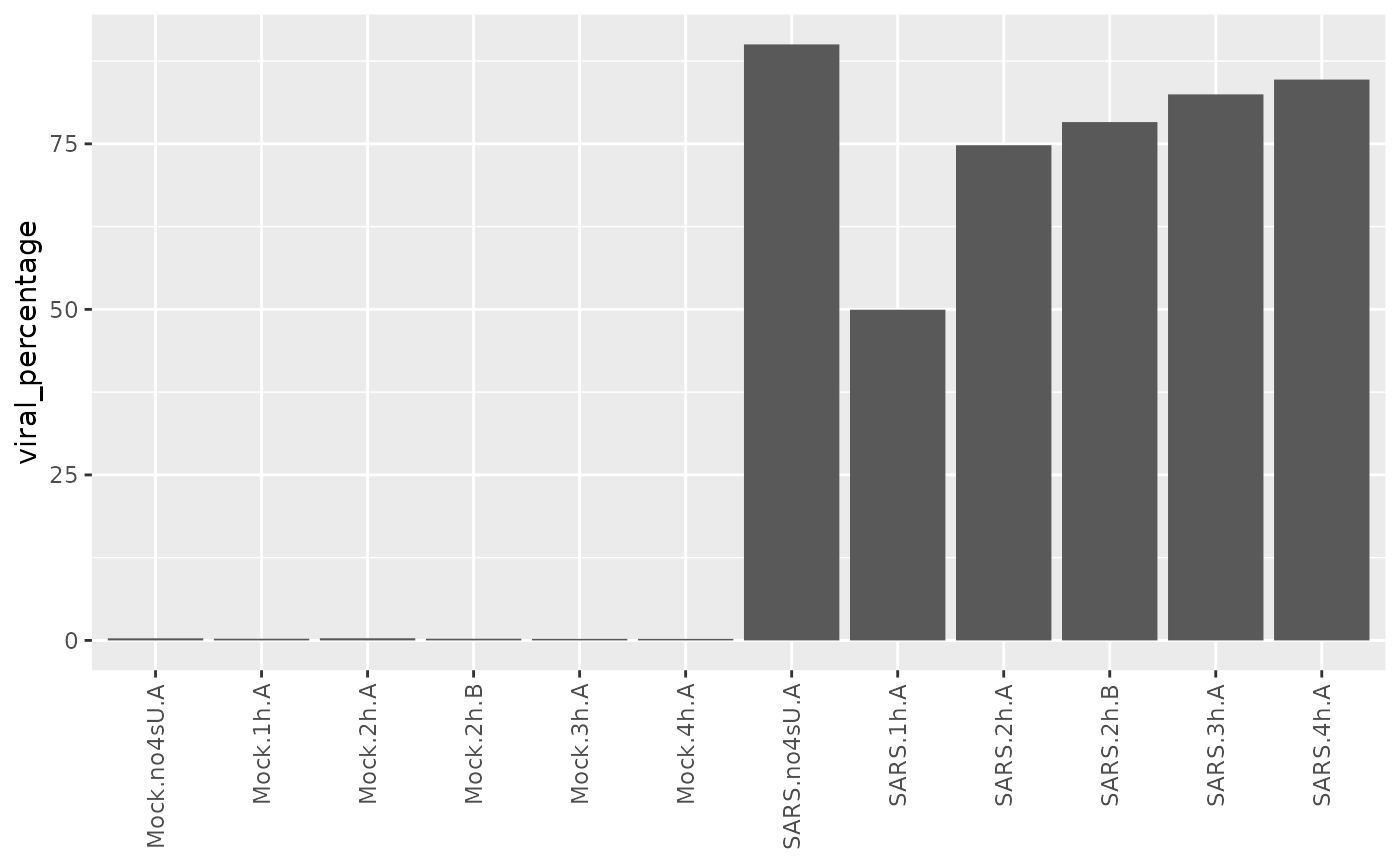
Interestingly the 4sU-naive sample shows more viral gene expression, suggesting that 4sU had an effect on viral gene expression.
Since this is such an important control, there is also a specialized plotting function built into grandR for that:
PlotTypeDistribution(sars,relative = TRUE)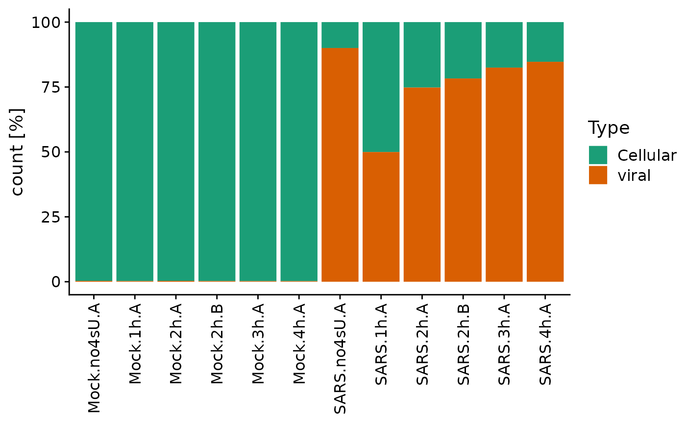
There is a column in the Coldata metadata table that has
a special meaning: Condition. It is used by many functions
as a default, e.g. to plot colors in the PCA or to model kinetics per
conditions. It can be accessed by it’s own function:
Condition(sars) [1] Mock Mock Mock Mock Mock Mock SARS SARS SARS SARS SARS SARS
Levels: Mock SARSand it can be set either directly:
Coldata(sars,"saved")<-Condition(sars)                  # save it for later use!
Condition(sars)<-rep(c("control","infected"),each=6)    # set new conditions directly
Coldata(sars)
Name Condition Replicate duration.4sU duration.4sU.original no4sU hpi
Mock.no4sU.A Mock.no4sU.A control A 0 no4sU TRUE 3hpi
Mock.1h.A Mock.1h.A control A 1 1h FALSE 4hpi
Mock.2h.A Mock.2h.A control A 2 2h FALSE 5hpi
Mock.2h.B Mock.2h.B control B 2 2h FALSE 5hpi
Mock.3h.A Mock.3h.A control A 3 3h FALSE 6hpi
Mock.4h.A Mock.4h.A control A 4 4h FALSE 7hpi
SARS.no4sU.A SARS.no4sU.A infected A 0 no4sU TRUE 3hpi
SARS.1h.A SARS.1h.A infected A 1 1h FALSE 4hpi
SARS.2h.A SARS.2h.A infected A 2 2h FALSE 5hpi
SARS.2h.B SARS.2h.B infected B 2 2h FALSE 5hpi
SARS.3h.A SARS.3h.A infected A 3 3h FALSE 6hpi
SARS.4h.A SARS.4h.A infected A 4 4h FALSE 7hpi
viral_percentage saved
Mock.no4sU.A 0.3188959 Mock
Mock.1h.A 0.2562894 Mock
Mock.2h.A 0.3261652 Mock
Mock.2h.B 0.2571997 Mock
Mock.3h.A 0.2354163 Mock
Mock.4h.A 0.2294342 Mock
SARS.no4sU.A 90.0177227 SARS
SARS.1h.A 49.9487279 SARS
SARS.2h.A 74.7904731 SARS
SARS.2h.B 78.2874060 SARS
SARS.3h.A 82.4704774 SARS
SARS.4h.A 84.7068470 SARSor from one or several columns of the metadata (here this this not really reasonable, but there are situations where combining more than one metadata column makes sense):
Condition(sars)<-c("saved","Replicate")   # set it by combining to other columns from the Coldata
Condition(sars)
[1] Mock A Mock A Mock A Mock B Mock A Mock A SARS A SARS A SARS A SARS B SARS A SARS A
Levels: Mock A SARS A Mock B SARS B
Condition(sars)<-"saved"                  # set it to one other column from the Coldata
Condition(sars)
[1] Mock Mock Mock Mock Mock Mock SARS SARS SARS SARS SARS SARS
Levels: Mock SARS